• Home
  • Readings
  • Github
  • MIES
  • TmVal
  • About
Gene Dan's Blog

No. 154: FASLR – The Bornhuetter-Ferguson Technique

3 August, 2025 5:10 PM / Leave a Comment / Gene Dan

FASLR v0.0.9 adds a third reserving technique, the Bornhuetter-Ferguson technique. From a technical standpoint, there wasn’t much work beyond adding a few more columns to what I had done with the expected loss technique, namely the percentage unreported and unpaid losses that serve as the credibility weighting between the development and expected claims techniques – the two methods that underlie the Bornhuetter-Ferguson method. So in this blog post, I’ll focus on the engineering decisions that expedited the turnaround time on this release – three weeks as opposed to the many months it took to develop the base loss model from which the core FASLR reserving techniques derive. It is this base model that enables newer techniques and future extensions to be quickly developed.

If you are new to FASLR, it stands for Free Actuarial System for Loss Reserving. If you are more interested in discovering FASLR’s capabilities, you can browse previous posts about the project on this blog. You are also free to browse the source code on the CAS GitHub or view the documentation on the project’s website.

The Base Model Class

The development goals of the recent past and near future involve incorporating the basic reserving methods from the Friedland reserving paper into the FASLR application, namely:

  1. Chain Ladder
  2. Expected Loss
  3. Bornhuetter-Ferguson
  4. Benktander
  5. Cape Cod

Creating the prototype for the chain ladder method was quick, mostly because it only involved the selection of the development factors and did not include features that are required for more advanced techniques such as trending, or summary exhibits such as IBNR and unpaid loss calculations. It became apparent by the time I worked on the Expected loss technique that not only would I need to create these new features, but also to engineer them in a way that allows them to be shared by the other models without having to recreate them from scratch every time. This would involve creating a base model class from which the other classes would inherit, speeding up development time and easing ongoing maintenance in the future. I hope this simple diagram shows you what I had in mind:

Base model inheritance diagram

I’m not going to pretend I know the rules of any diagramming standards (I don’t), but I hope this one is simple enough for you to get the idea. The base model serves as a template from which other models derive, this includes features for:

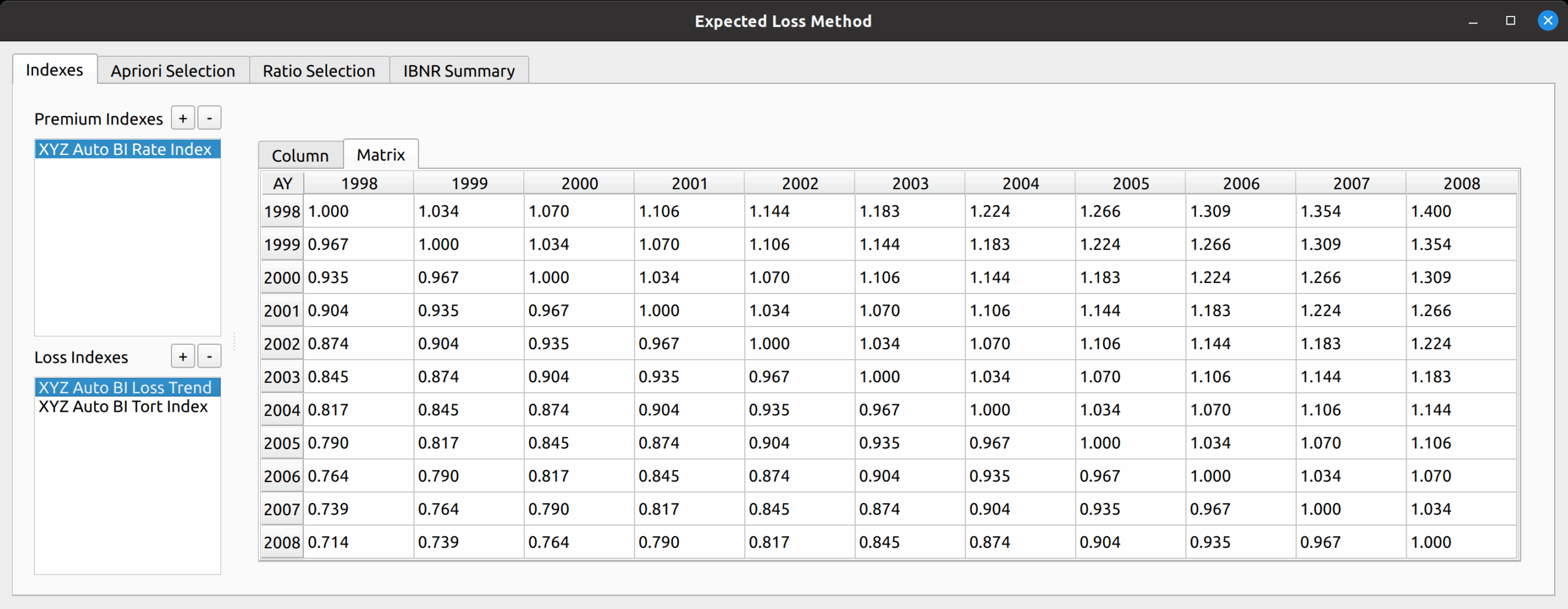
  • The display of loss triangles
  • Trending of losses and premiums
  • Selection of some kind of ratio (e.g., link or loss ratios)
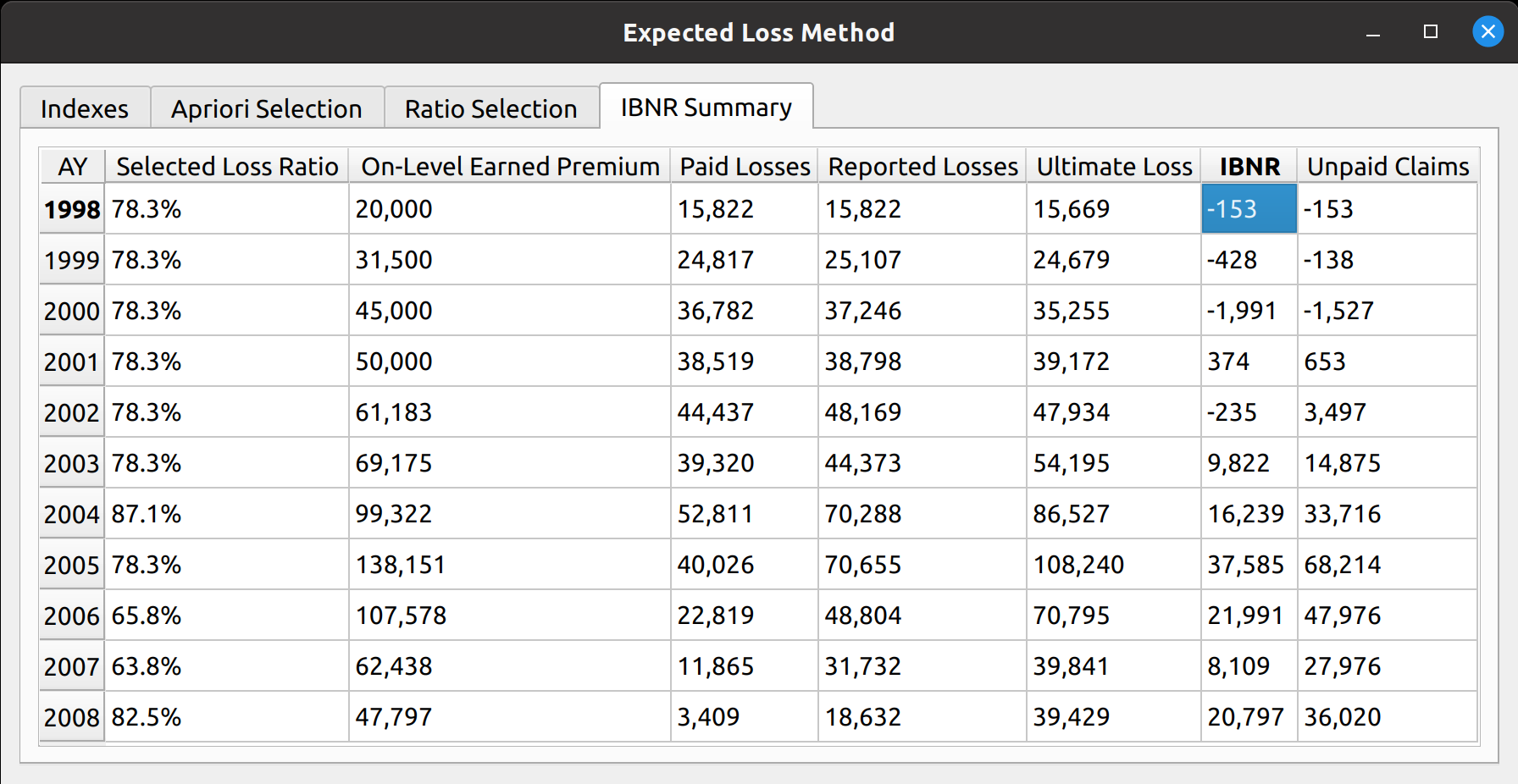
  • Ultimate loss and IBNR summaries

These are listed to the right of the base model in the diagram. The models listed below inherit these features by default, although they can be overridden with model-specific tweaks. For example, the chain ladder technique involves the selection of link ratios whereas the expected loss and other techniques involve the selection of both link and loss ratios. Furthermore, model-specific features are listed below the models, like how the Bornhuetter-Ferguson technique adds a credibility calculation using unpaid and unreported loss percentages.

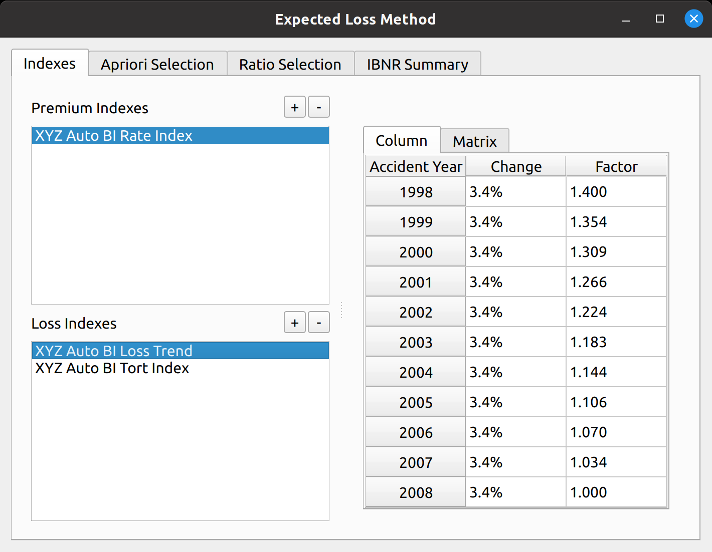
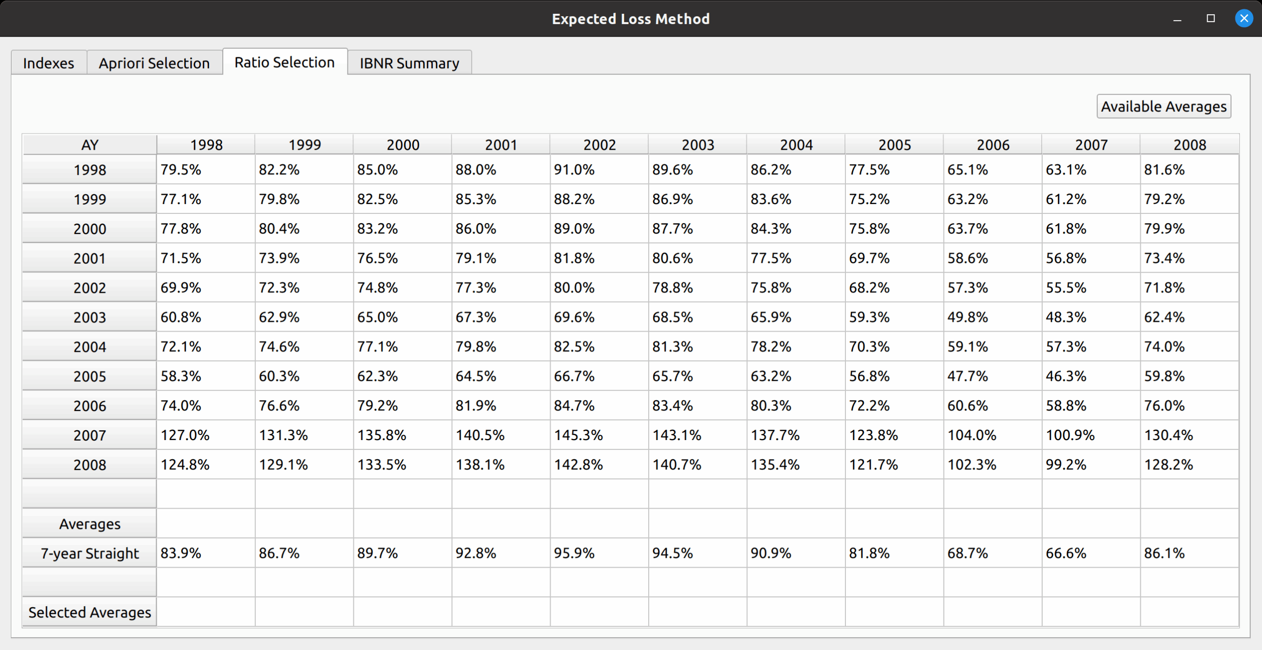
The Ratio Selection Model

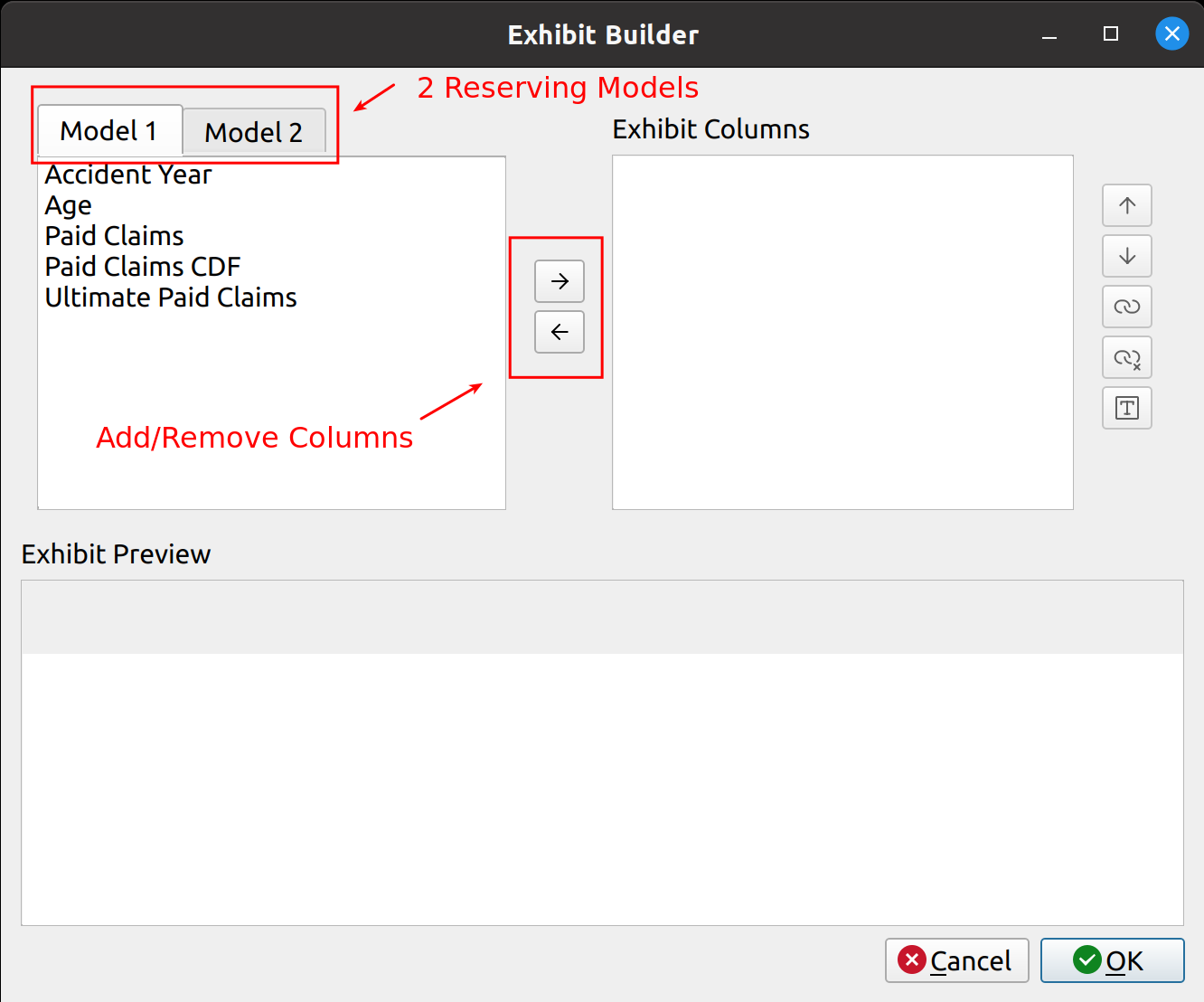
At the heart of the base model is the selection of ratios. This can be any kind of ratio, such as link ratios in the chain ladder method or loss ratios in the expected loss method. Below is a picture of the bare bones, base ratio selection model.

The base ratio selection model.

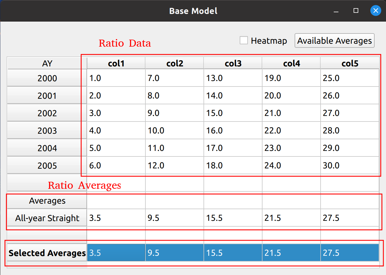
You can see that the data don’t mean anything, as the base model alone cannot serve as a true reserving model – method specific tweaks are required. In a way, putting nonsense data as a placeholder will serve to demonstrate the base model’s flexibility in being used by the inheriting reserving models. You can see the features from this base model image that will be found in the inheriting models, such as:

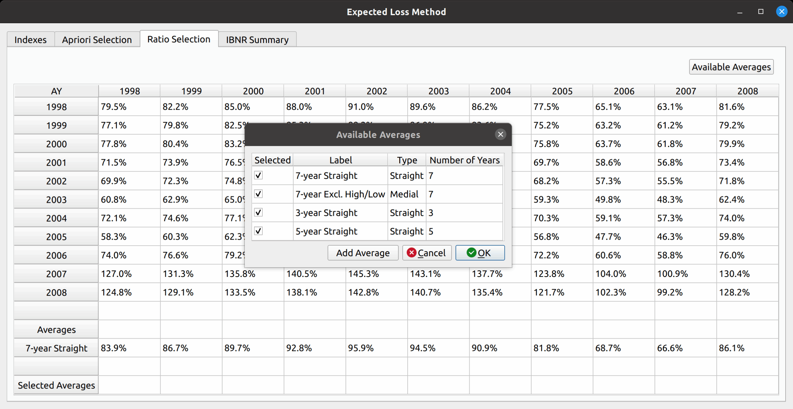
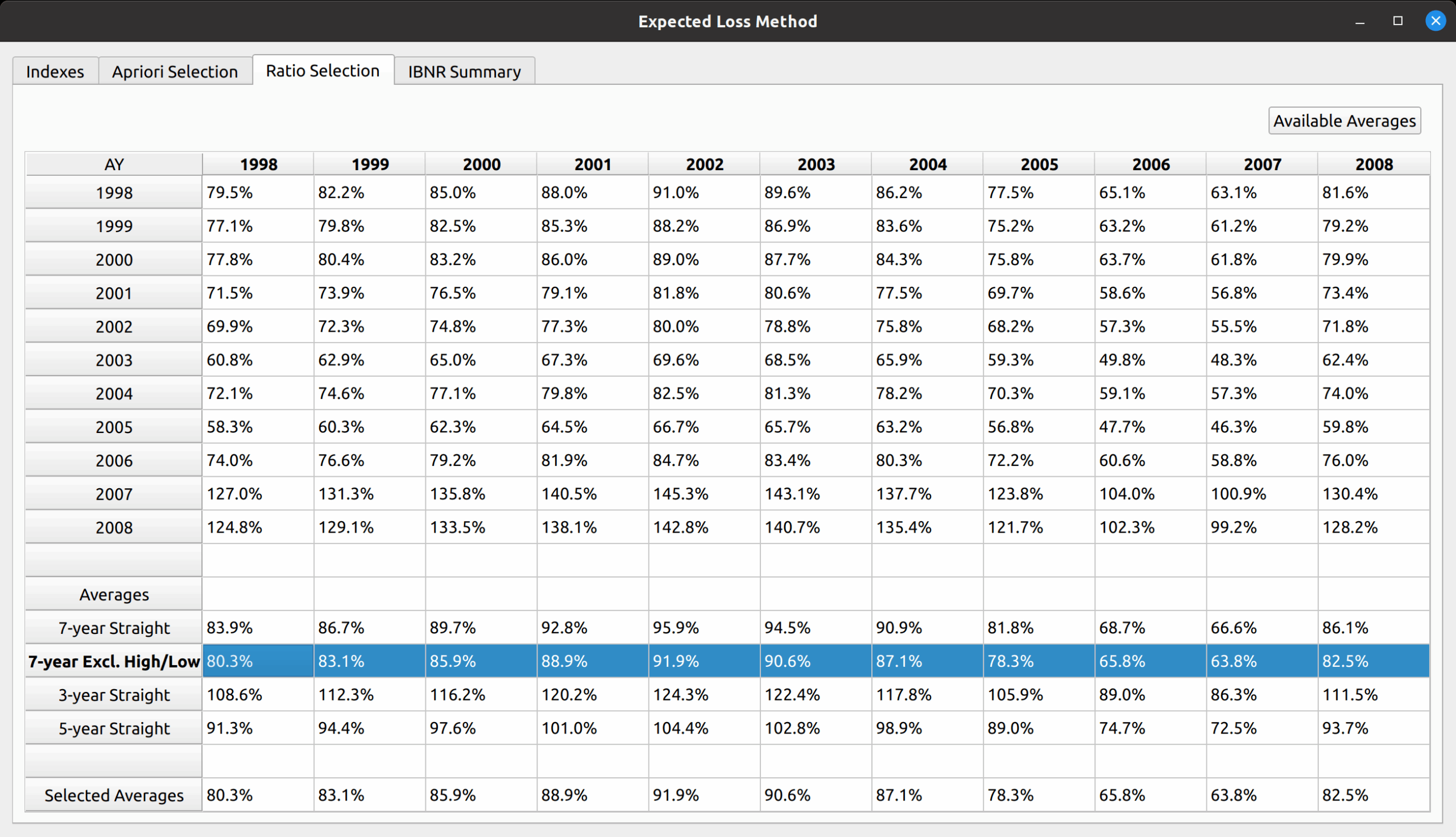
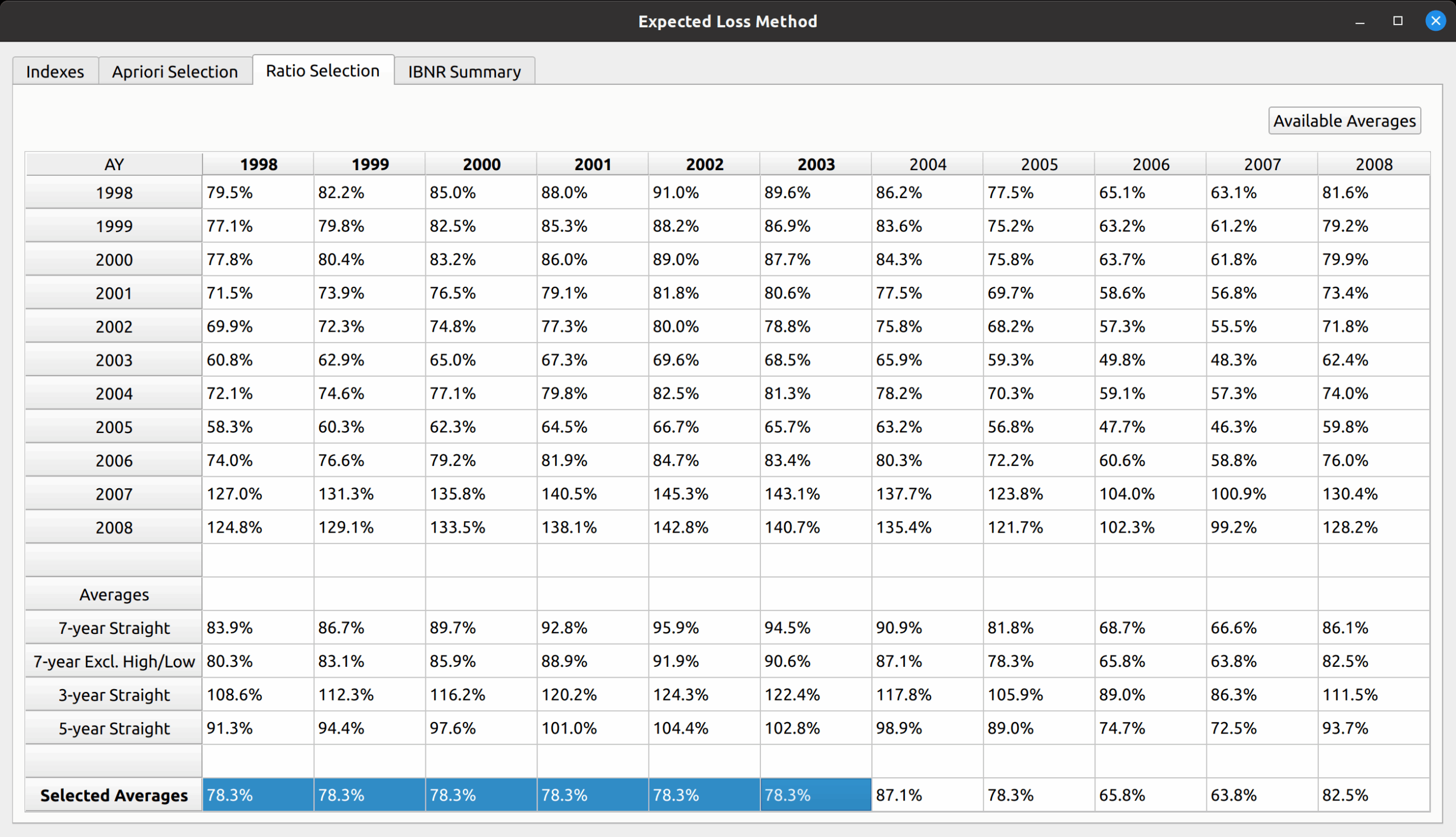
  • A toolbox at the top to toggle a heatmap and add average types
  • A DataFrame in the middle to hold ratio data
  • A section below the DataFrame to calculate averages common to various models (i.e., volume-weighted, straight, etc.)
  • A section holding the selected averages

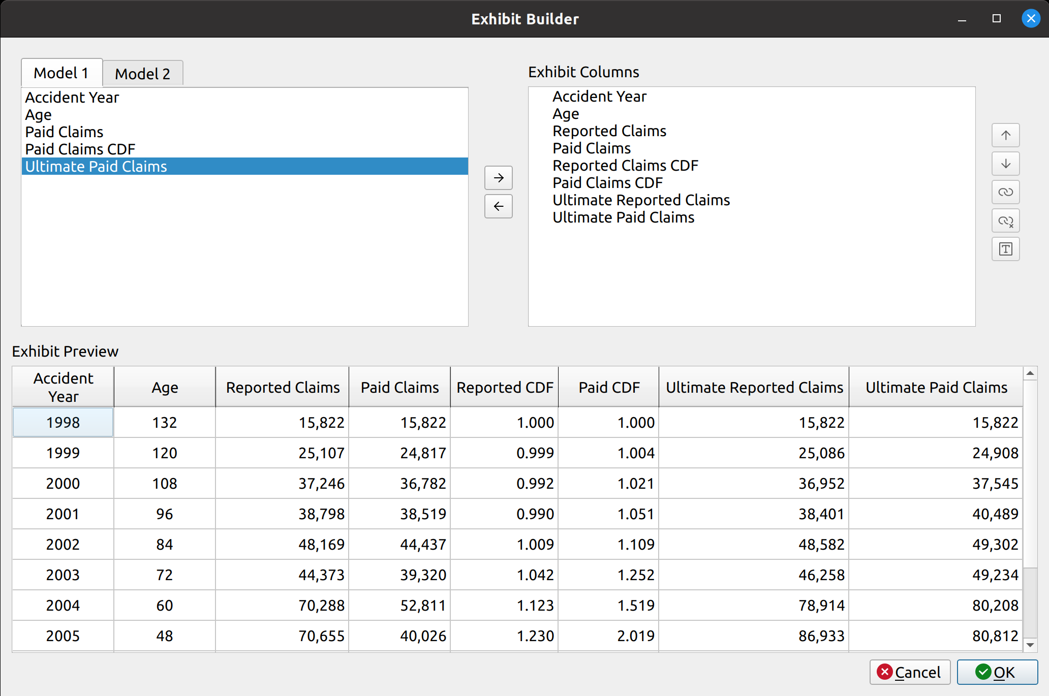
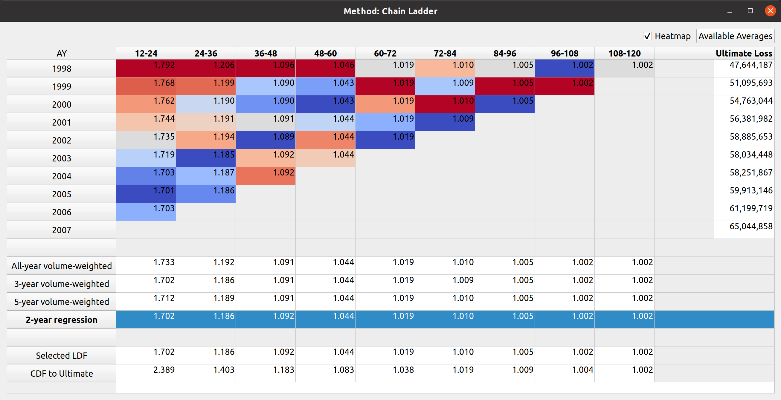
An example of the Chain Ladder model, which inherits from the base model, shows the heatmap feature applied as well as an auxiliary ultimate loss column:

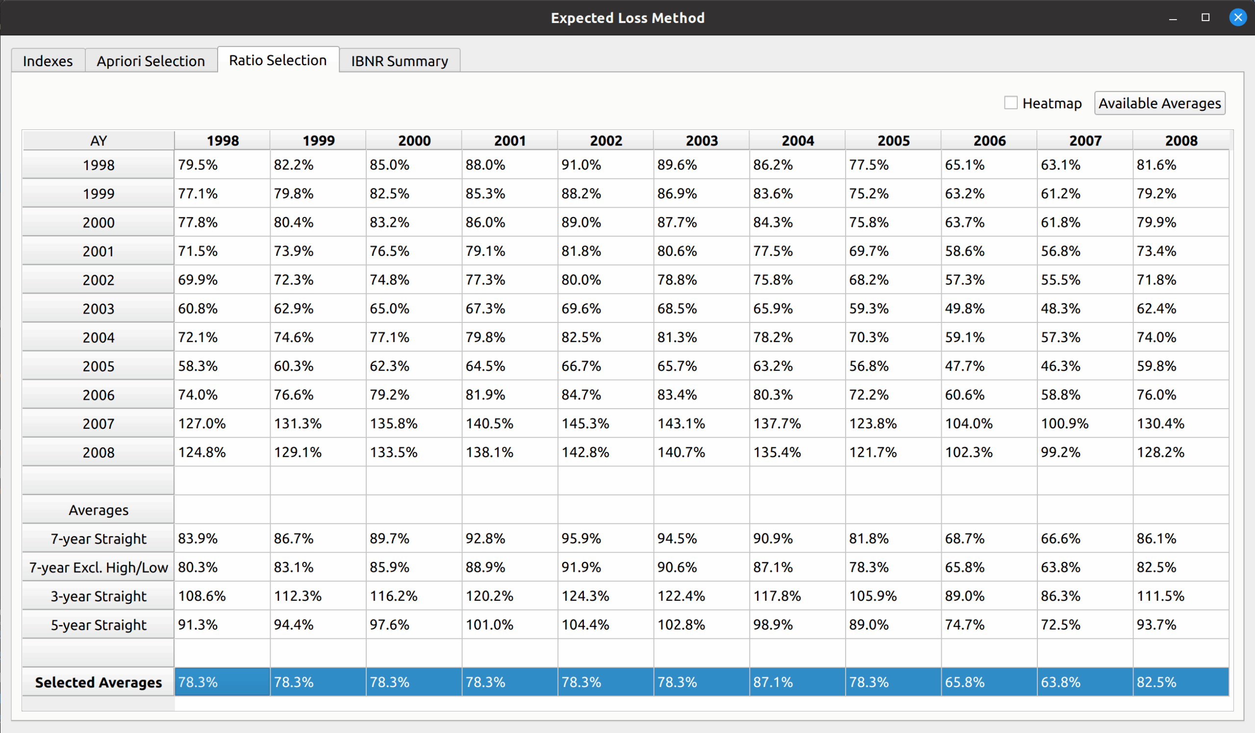
Another example is the expected loss model, which replaces the DataFrame with loss ratios instead of link ratios, and you can see that all the main sections described in the base model are still preserved:

Extensibility

A key motivation for the base model is to enable FASLR to accept custom user extensions. Due to the vast array of insurance products, and the nuances of the different reserving practices used between actuaries, it is impossible for an out-of-the box application to meet all the needs of all the users. By providing a base model class with a standard API, the user will be able to create their own subclasses of the base model, which will be accepted by FASLR so long as key aspects of the standard API remain intact.

For example, an actuary may have their own unique way of calculating expected claims to be used in the Borhnhuetter-Ferguson technique that is not offered by default in FASLR. If they create their own version of the base model, and match the API for exporting things like ultimate losses, they will be able to incorporate it into FASLR as a custom extension.

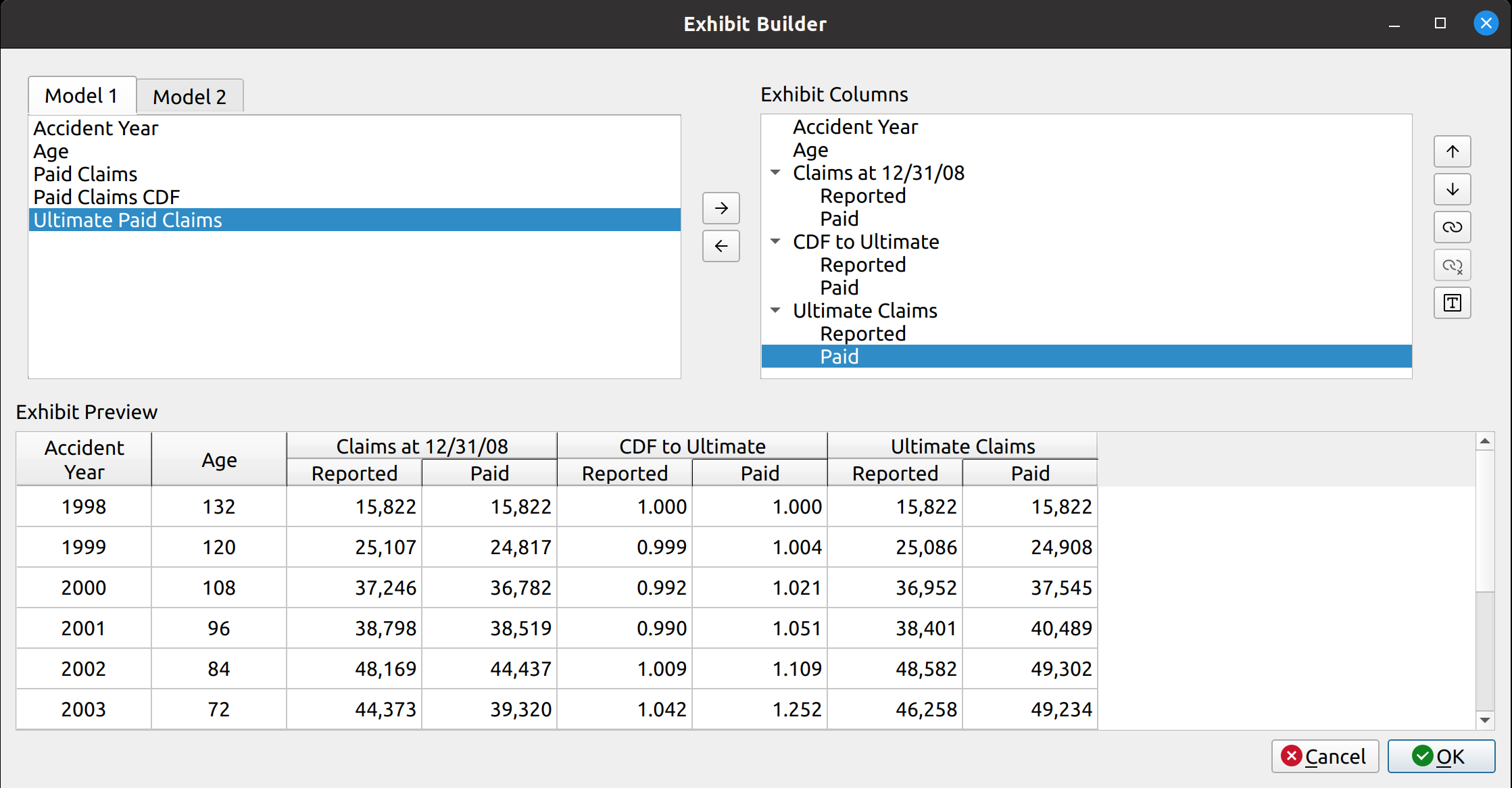
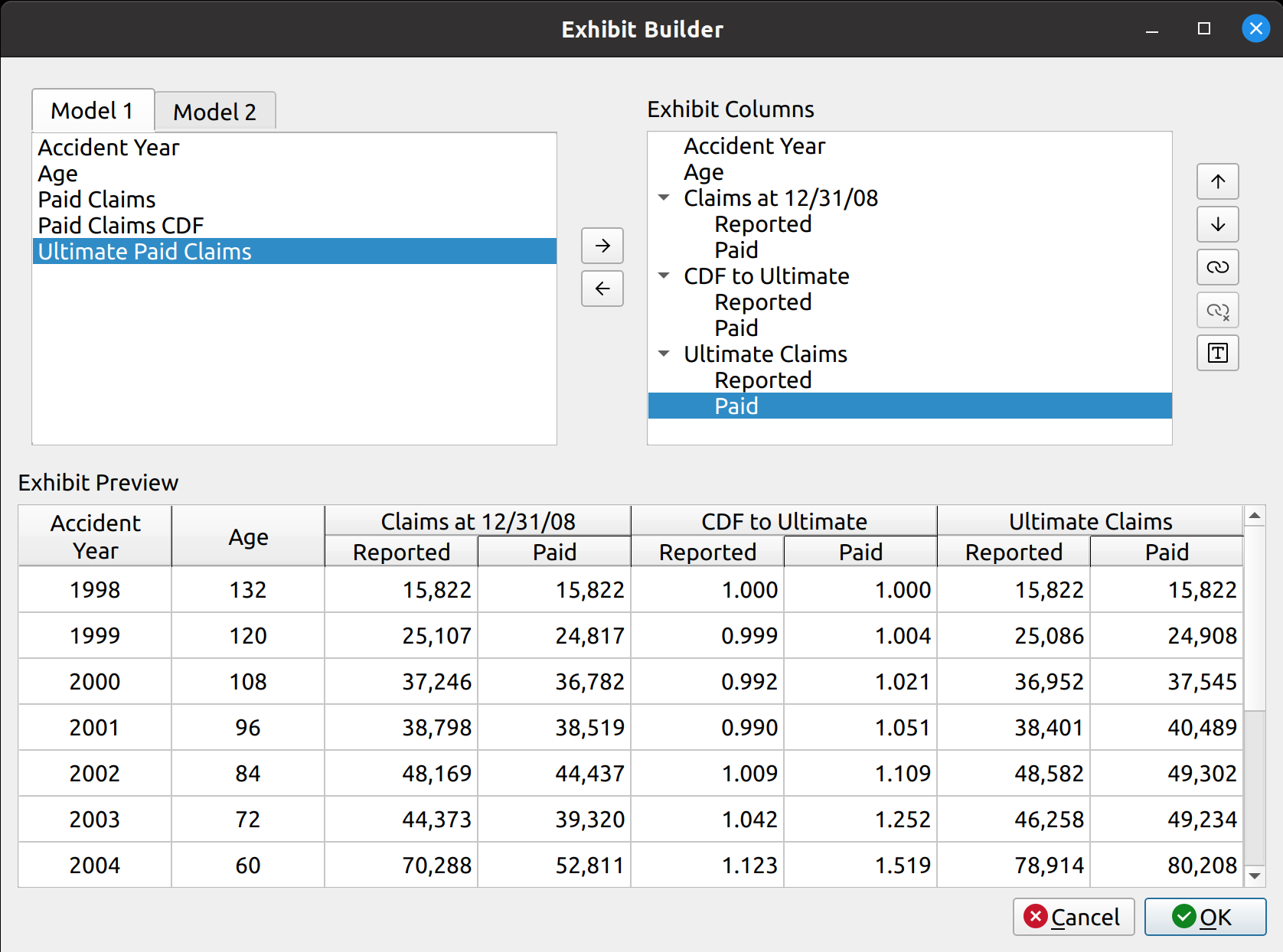
The Bornhuetter-Ferguson Widget

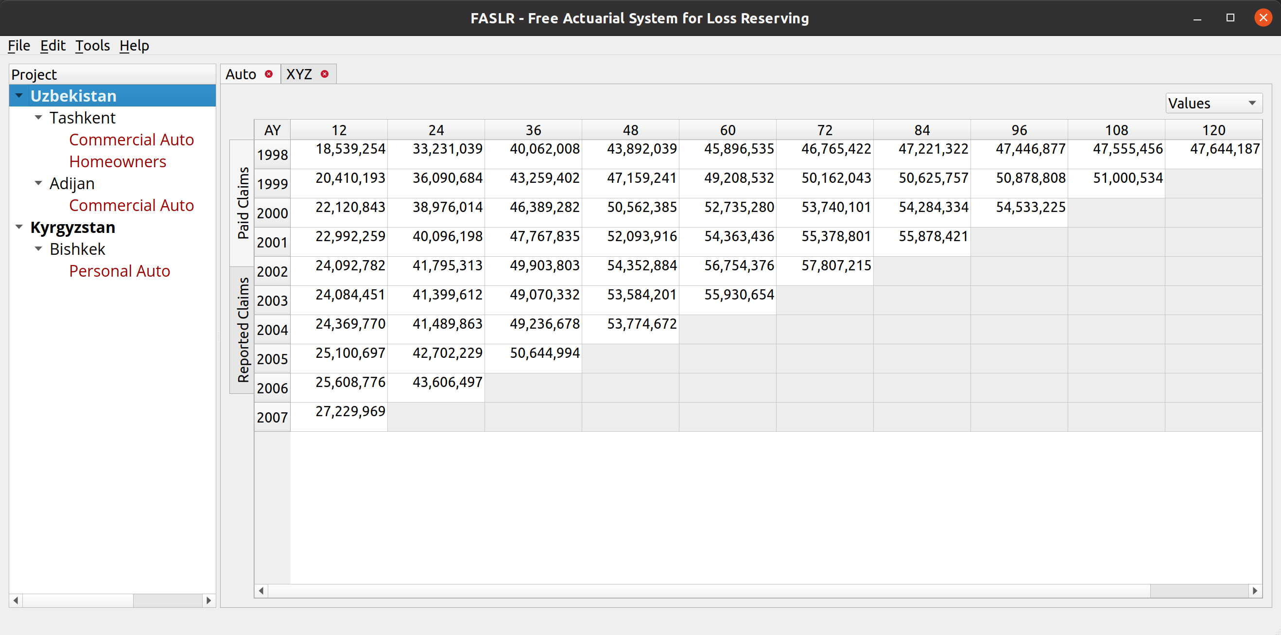
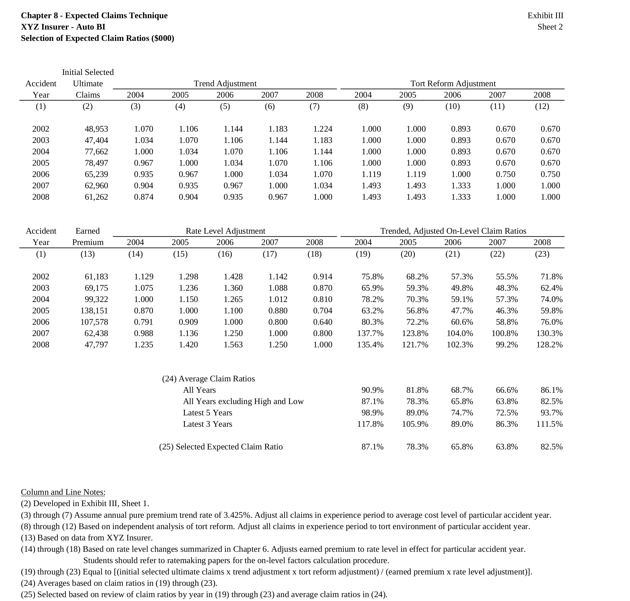
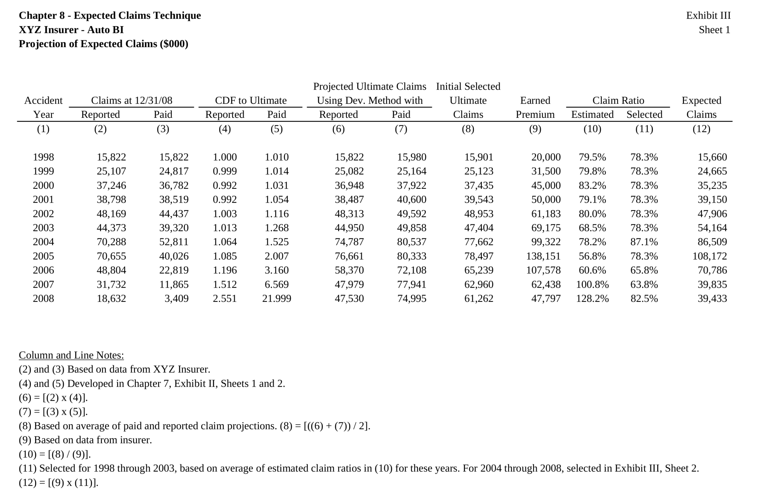
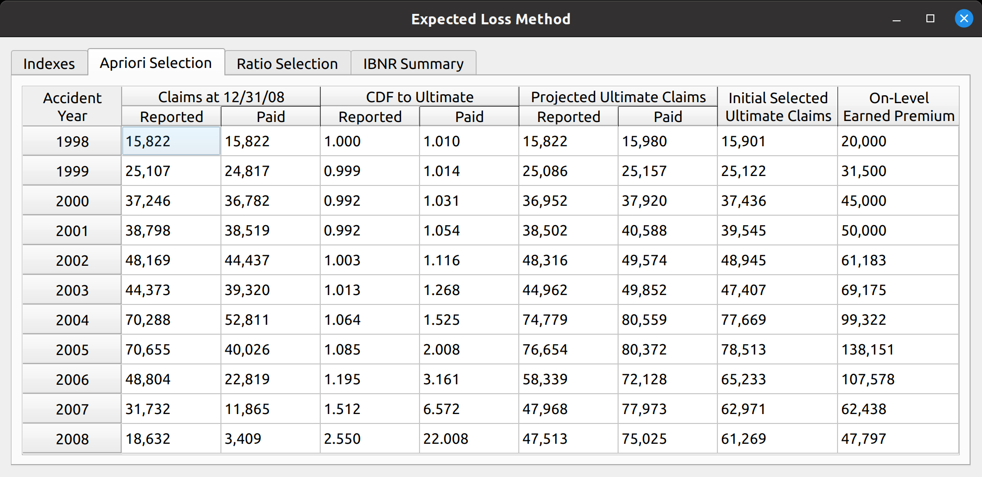
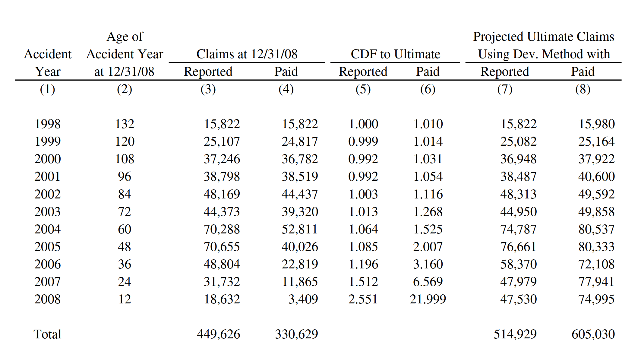
The next test of base model is to see if the Bornhuetter-Ferguson widget can inherit the features from the base model, and then incorporate the credibility calculations. In this example, we seek to replicate the XYZ Auto example from Friedland:


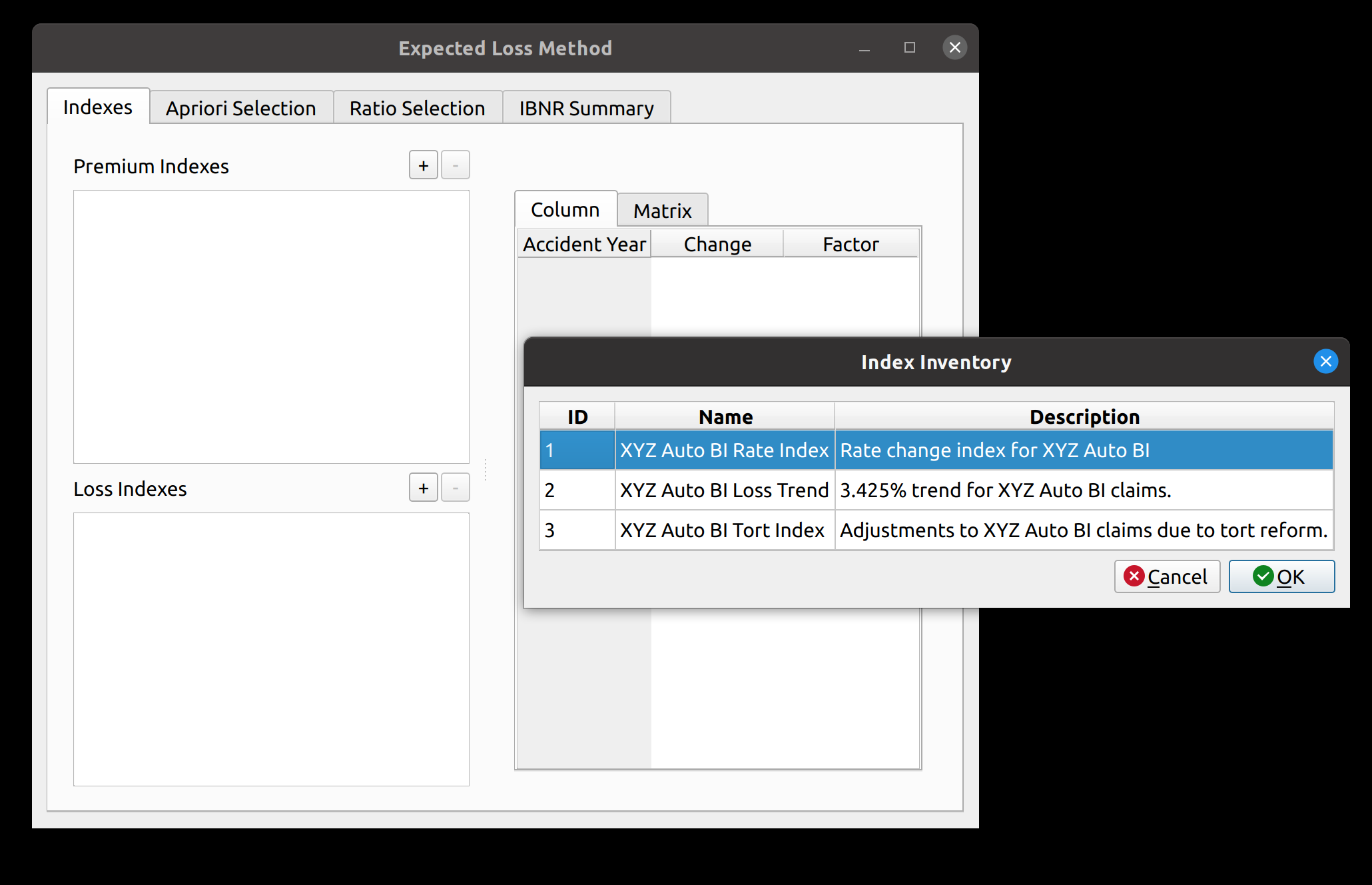
The widget is displayed below. The model uses almost all the features of the expected loss model: indexes an apriori selection of ultimate losses, and a selection of expected claims (note that my values differ slightly due to different rounding practices).

Posted in: Actuarial, FASLR

No. 153: FASLR – The Expected Loss Technique

13 July, 2025 1:29 PM / 1 Comment / Gene Dan

The release of FASLR v0.0.8 incorporates a second loss reserving technique into the application – the expected loss technique. This technique is commonly used to estimate ultimate losses for new lines of business or those for which we do not have much data. It’s been a long time since my last update, but I’m excited to continue a project that, besides being used to pad my resume, has brought me into contact with some interesting and innovative members of our profession.

For those wondering what I’ve been up to last year, I spent a good chunk of it writing my first paper for the CAS – Practitioners’ Guide to Building Actuarial Reserving Workflows Using Chainladder-Python, co-authored with John Bogaardt and Kenneth Hsu.

If you are new to FASLR, it stands for Free Actuarial System for Loss Reserving. If you are more interested in discovering FASLR’s capabilities, you can browse previous posts about the project on this blog. You are also free to browse the source code on the CAS GitHub or view the documentation on the project’s website.

Background

By itself, the expected claims technique is simple – it involves an apriori expectation (aka guess) on what ultimate losses will be, and then derives the IBNR estimate by subtracting the incurred losses to date. In its purest form, it can simply be a straight up guess as to what the ultimate losses are, but from a practical standpoint (and to make actuarial exams more challenging) there are some variations on the technique that make use of the observed claims to have some grounding in reality.

To include this technique as a new feature in FASLR, I adapted Friedland’s example that applies the techinque to an Auto BI line of business at an insurer named XYZ. I chose this example because it has several characteristics that make it well-suited for testing in a real-world environment:

  1. A mixed selection of loss ratios using a blend of loss ratio averaging techniques.
  2. The use of premium and loss trends, a feature which can also be applied to other techniques.
  3. Incomplete values in the loss triangles.
  4. The application of the technique over all accident years, as opposed to just a single year (as seen in other examples in the text).

The most challenging part of this exercise was reproducing Friedland’s application of premium and loss indexes, which, from the paper, was difficult to interpret since it involves 2-dimensional indexes, bringing each accident year to the level of every other accident year.

Friedland Exhibit III, Sheet 2

Below, is the exhibit that we seek to reproduce, which shows the selection of initial and final ultimate losses, with some modifications to enhance the user experience. Note that my numbers will differ slightly from hers due to differing rounding practices between her paper and my application.

Friedland Exhibit III, Sheet I

Trending

FASLR v0.0.8 adds a loss and premium trending widget. The widget has 2 main subsections. The subsection to the left of the splitter contains two list views that allow us to add premium and loss indexes, respectively. The subsection to the right of the splitter allows one to preview the index(es) that they have added. The plus/minus buttons open up a dialog from which we can insert indexes to the model. This list shown within the dialog box is obtained by querying a database that contains all the indexes uploaded to the application.

Adding trends

For our example, we add one premium trend index, and two loss indexes: a 3.425% Auto BI loss trend and an index to adjust losses for tort reform. Once this is done, the preview section gets populated. The preview section has two tabs to visualize the adjustment factors. The “Column” tab shows the factors to bring each accident year to the level of the latest accident year.

Previewing trends

The “Matrix” tab shows the index in matrix form, showing a 2-dimension array of factors to bring each accident year to the level of every other accident year as required for Friedland’s example.

The matrix preview view of an index.

This variation of the expected loss method involves first selecting an initial set of ultimate claims, a straight average of the ultimate losses generated by the chain ladder method applied to paid and reported losses. I have made my own stylistic departure from Friedland’s example by moving the next step – the selection of loss ratios, to the subsequent tab of the model widget.

The apriroi ultimate loss selection.

In the next section, the “Ratio Selection Tab”, the trends that we added to the model are applied to the premiums and initial ultimate losses to produce a matrix of loss ratios.
Just like with the chain ladder method, we then produce various averages to help us select our set of apriori loss ratios. The default is the 7-year straight average. Note that this differs from Friedland’s exhibit as my version incorporates more accident years.

The ratio selection widget.

To reproduce Friedland’s exhibit, we can add additional averages by pressing the “Add Averages” button in the upper-right hand corner. This opens a dialog box that lets us add the 7-year medial, 5-year straight, and 3-year straight. In addition to those shown in the table, the model allows us to create new average types (such as a 4-year average, if one desires).

Adding loss ratio average types.

Just like the paper, we first select the 7-year medial average, which copies those averages to the “Selected Averages” row.

Selecting the 7-year straight average.

We then complete the reproduction of Friedland’s results by manually inputting the 1998-2003 volume-weighted loss ratio for those years. This can be done simply by copying 78.3% to the corresponding cells.

Overriding the 1998-2003 accident year averages with the 78.3% volume-weighted average.

IBNR Summary

The last exhibit, accessed via the IBNR Summary tab, calculates the IBNR by subtracting incurred losses from ultimate losses, and produces an unpaid claim estimate by subtracting paid losses from ultimate losses.
The IBNR summary.

Posted in: Actuarial

No. 152: FASLR – Automated Testing with pytest

4 September, 2023 8:39 PM / Leave a Comment / Gene Dan

The release of FASLR v0.0.7 introduces a test suite to ensure the accuracy of calculations. A test suite is a sub-package or collection of files that runs the project’s code against a set of expected inputs, and compares the generated outputs to a set of expected outputs. For example, one of the tests may run the chain ladder method against a sample dataset to make sure the resulting ultimate losses a calculated correctly. This test is then run whenever we make code changes to the project. In this manner, we can check that FASLR continues to work correctly as the project matures.

If you are new to FASLR, it stands for Free Actuarial System for Loss Reserving. This update has more of a project management-related focus, so if you are more interested in discovering FASLR’s capabilities, you can browse previous posts about the project on this blog. You are also free to browse the source code on the CAS GitHub or view the documentation on the project’s website.

Motivations

What motivated this update, focusing on the development workflow rather than adding new features, was that certain packages that the project depends on, such as pandas and sqlalchemy, have become out-of-date. Although I had the option of simply upgrading all of the packages without running the code against a test suite, I figured the time has come to add one since the project was growing in complexity and has picked up some interest from people other than myself, so there was the need to make sure that further updates to the project would not break its existing functionality.

My IDE telling me my dependencies are out of date.

FASLR’s sister project, chainladder-python, has had a working test suite for several years now, so adding one would demonstrate that the project aims to deliver on quality, and further cement the CAS GitHub as a guide for other actuaries on how to properly use Python, write libraries, and deploy software in their own careers.

Preventing Errors

When an actuary assesses the accuracy of a project, not just one involving code, but anything involving computations – they tend to ask themself the following questions:

  • How do I know my formulas are correct?
  • If I make changes, how can I make sure they don’t break existing computations?
  • If more people join the project and start contributing, how can I integrate their changes without messing things up?

If you have ever done a data reconciliation, or added a spreadsheet to check premium and loss totals against your data source, then you have already performed some testing on your work. If any changes to your project were to break your reconciliation sheet or lead to odd totals, then the change has broken your project. The motivations behind a software testing suite are no different – except instead of adding extra formulas to a spreadsheet, we add extra lines of code to a project.

Building a Testing Suite

There are several ways to build a test suite – for example, you may choose to write your own custom functions to test critical parts of your code or you can use a framework such as unittest or pytest. A framework, usually implemented in the form of a package, can make the testing process easier by providing a standardized way to separate test code from feature code, running the entire test suite or specified parts of it, or reducing redundancy by enabling test functions to run multiple times using different input data sets.

I chose to use pytest, partly because chainladder also uses it, and also because members of the Python community recommend it. Writing a test suite for FASLR also has the complication of having to test GUI components, which unlike testing a package, involves testing visual features such as button clicks, key presses, and menu selections. In order to do this, I used a package called pytest-qt, which invokes a bot to simulate user actions. For example, this bot can be used to enter a custom development factor into a field and then pytest can use that value to see if it correctly flows through the intended calculations.

Automating tests with GitHub Actions

FASLR combines pytest with GitHub Actions to automatically run its test suite upon certain events, such as when changes are pushed to the repo, or when someone opens up a pull request, allowing me to make sure their proposed changes won’t break the program.

Code Coverage

One question that arises when building a test suite is – how do I know I’ve written enough tests? Although I don’t believe there is a bulletproof way to prevent all bugs, there are certain metrics we can use to gain comfort and convince others that we have put in a good faith effort to do so. One such metric is code coverage, which is the percentage of lines of your project that the test suite has run. For example, if a project has 95% code coverage, 95% of the source code was executed by the test suite. This does not mean your code is 95% bug free, just that 95% of it has been executed. This also does not mean that your tests were well-thought out or that you correctly anticipated that parts of the code that needed the most testing. It can however, help to identify glaring holes in your package that you may have omitted from testing.

FASLR uses codecov, a third-party product that integrates with GitHub and hosts your project’s coverage reports. In the image below, we can see that our test suite has covered 92% of our code:

A coverage report can provide detail as to which files are completely covered, and which files need further testing. The example below shows some of the output from pytest:

To view the codecov summary on FASLR, click here.

Other Updates

FASLR v0.0.7 has added some further updates, in addition to the test suite:

  • An improved heatmap function, written by P. Sharma
  • Automated documentation deployment via GitHub Actions
  • Schema documentation page on the FASLR website
  • A development chatroom, on Gitter
Posted in: Actuarial

No. 151: FASLR – Exhibit Builder

19 February, 2023 3:35 PM / Leave a Comment / Gene Dan

The release of FASLR v0.0.6 adds an exhibit builder to assist the actuary in comparing output between models and making ultimate selections. Usually, when an actuary conducts a reserve study, they will employ a variety of models using different actuarial methods to estimate the ultimate value of losses. The reason why this is done is because no single model is a perfect representation of reality – each method comes with its own strengths and weaknesses. By offering a way for the user to develop custom exhibits to make comparisons between those models, FASLR (Free Actuarial System for Loss Reserving) enables the actuary to balance these trade-offs to select what they believe to be their best estimate of ultimate losses.

Furthermore, I wanted to make sure the user had the ability to fully customize their reports. Otherwise, static reports would limit the capabilities of FASLR and give users the urge to export things to Excel to make up for its shortcomings – something all too common with financial software. By enabling customization, I hope to not only drive long-term user engagement, but also to make the reserving experience as pleasant as possible.

Although this feature may appear to be mundane compared to those involving sophisticated actuarial methods, it is nonetheless an essential part of FASLR and was the most difficult thing to design so far in the lifespan of the project. The reason why is because Qt did not provide a native way to display hierarchical headers, which are commonly found in Excel-based financial reports. In researching how to implement this via subclassing, I came across a post on stack overflow where another user achieved this using C++, for which I am grateful. I was able to port his solution over to Python, but understanding what he did and then translating the language took about three weeks to do. Furthermore, many of the column manipulation features I wanted to add were difficult to pull off – with still more bugs for me to handle in the near future.

Thankfully, I was able to get a prototype running that demonstrates most of what I wanted to achieve, showing that FASLR can one day do important things, provided I have the time to polish it up. Today, I will demonstrate how it works by replicating a result from the Friedland reserving paper.

As usual, feel free to browse the documentation or the source code hosted on the CAS GitHub page.

Basic Layout

The exhibit builder has three main components:

  1. Model Columns
  2. Exhibit Columns
  3. Exhibit Preview

The Model Columns are located as a tab widget in the upper left-hand corner. Here we have two models, each of which has a variety of components available, such as year, age, CDFs, losses, etc., that can be included in a report.

The Exhibit Columns is the list box in the upper-right hand corner. These are the columns selected from the model that will be displayed in the exhibit.

The Exhibit Preview is the table at the bottom. This displays the columns listed in the Exhibit Columns box in the form of a table, to let the user preview what their report will look like.

Example Demonstration

Consider the following exhibit from the Friedland text. Here, we are trying to project ultimate claims, and we have constructed two models using the chain ladder method – one using paid claims, and the other using reported claims.

Now, I will demonstrate how we can replicate this exhibit in FASLR. My values won’t match exactly. There are some tail factors from the text that I am not including here, and some rounding errors will produce slightly different numbers anyway. My main focus is just getting the overall layout of the report right.

The big challenge, as mentioned before, was making the hierarchical headers. For example, in the image above, columns (3) and (4) have two levels of headers – the topmost header “Claims at 12/31/08” groups two headers below it, “Reported,” and “Paid.” Data formatted for human reading are often structured differently than those used for mathematical analysis, and the use of features such as hierarchical headers makes things easier to understand for the person. One of FASLR’s features for exhibits enables the user to group columns together in this fashion.

Column Selection

First, we start with a blank Exhibit Builder. The two tabs, labeled Model 1 and Model 2, contain the available components from two fitted models, a paid chain ladder model and a reported chain ladder model, respectively. In the middle, we may use the arrow buttons to add or remove columns from the exhibit. To do this, we click on the columns we want from the tabs and then click the right arrow button:

You can now see that the Exhibit Preview gets populated with data from these selected columns.

Grouping Columns

Now We have the right columns, but the headers are unorganized and a bit verbose. Now we can make the hierarchical headers. I call these headers column groups. To make a column group, highlight the columns you want to group from the Exhibit Columns list, and press the “link” button on the right-hand side. A box will pop up asking you to come up with a name for the column group:

Now we can see that the headers have changed into the hierarchical groupings that we specified:

Also, the Exhibit Columns list is now organized as a hierarchical tree, rather than just a flat list.

Renaming Columns

Although we have our column groupings, the sub column labels are too verbose and redundant. We can simplify these by renaming them. To do this, press the “T” button on the right-hand side:

After doing this, we now have the desired exhibit:

Summary

The following video shows the entire process:

https://genedan.com/wp-content/uploads/2023/02/Screencast-from-02-19-2023-041802-PM.webm
Posted in: Actuarial

No. 150: FASLR – Tail Factor Analysis

22 January, 2023 5:07 PM / Leave a Comment / Gene Dan

The release of FASLR v0.0.5 adds a new tail factor analysis pane. Tail factor analysis is a way to estimate the extent to which development will occur beyond the latest age of the triangle, and is an essential part of the process of estimating insurance liabilities (or other longitudinal things that need estimating).

Creating the pane was quite challenging, as doing so introduced several design problems that I hadn’t experienced before. These would include the need to not only display charts in a PyQt application, but to also dynamically update them as user inputs change. I also had to consider that most users will want to make a tail selection from one out of several tail factor models, so there was the need to be able to simultaneously accommodate multiple models within a single window without being aesthetically overwhelming.

As usual, feel free to browse the documentation or the source code hosted on the CAS GitHub page.

Basic Layout

The new tail pane has two main parts. The left side accepts user input, and the right side displays a series of diagnostic charts that automatically update depending on what the user chooses.

Tail Candidates

When an actuary conducts a tail study, they will often create several models and then make a selection after weighing the various trade-offs between the models. I call these models tail candidates, and these are organized in the tail pane via tabs on the left side. The user can press the +/- buttons located to the right of the tabs to add or remove candidates. Below, the user has created 5 candidate tails to choose from:

To switch between the candidates, the user just needs to click between the tabs.

Supported Methods

The FASLR tail pane supports the same methods as those from the underlying chain ladder package:

  • Constant
  • Curve
  • Bondy
  • Clark

The user chooses the method by selecting a radio button, which then updates a form below it depending on the selection. For example, the curve method takes user input for the regression parameters:

Charts

The tail pane comes with a handful of diagnostic charts that automatically update when the user adds or removes tail candidates, or changes any of the inputs. These charts can be toggled by pressing the buttons on the right side of the tail pane. For example, the image below shows a simple bar chart comparing the tail factor between candidates:

Lastly, the user can select which tail candidate they want to use by clicking the checkbox at the bottom, “Mark as selected”:

Posted in: Actuarial

Post Navigation

1 2 3 … 30 Next »

Archives

  • August 2025
  • July 2025
  • September 2023
  • February 2023
  • January 2023
  • October 2022
  • March 2022
  • February 2022
  • December 2021
  • July 2020
  • June 2020
  • May 2020
  • May 2019
  • April 2019
  • November 2018
  • September 2018
  • August 2018
  • December 2017
  • July 2017
  • March 2017
  • November 2016
  • December 2014
  • November 2014
  • October 2014
  • August 2014
  • July 2014
  • June 2014
  • February 2014
  • December 2013
  • October 2013
  • August 2013
  • July 2013
  • June 2013
  • March 2013
  • January 2013
  • November 2012
  • October 2012
  • September 2012
  • August 2012
  • July 2012
  • June 2012
  • May 2012
  • April 2012
  • March 2012
  • February 2012
  • January 2012
  • December 2011
  • September 2011
  • August 2011
  • July 2011
  • June 2011
  • January 2011
  • December 2010
  • October 2010
  • September 2010
  • August 2010
  • June 2010
  • May 2010
  • April 2010
  • March 2010
  • September 2009
  • August 2009
  • May 2009
  • December 2008

Categories

  • Actuarial
  • Cycling
  • FASLR
  • Logs
  • Mathematics
  • MIES
  • Music
  • Uncategorized

Links

Cyclingnews
Jason Lee
Knitted Together
Megan Turley
Shama Cycles
Shama Cycles Blog
South Central Collegiate Cycling Conference
Texas Bicycle Racing Association
Texbiker.net
Tiffany Chan
USA Cycling
VeloNews

Texas Cycling

Cameron Lindsay
Jacob Dodson
Ken Day
Texas Cycling
Texas Cycling Blog
Whitney Schultz
© Copyright 2026 - Gene Dan's Blog
Infinity Theme by DesignCoral / WordPress