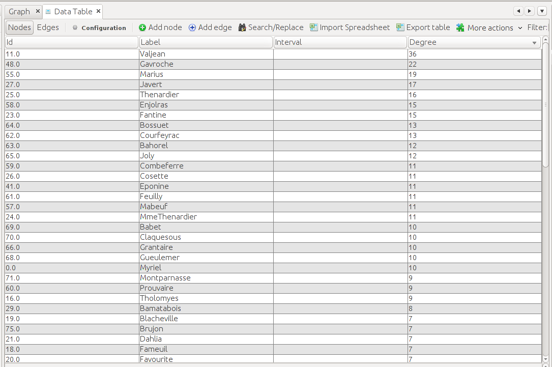
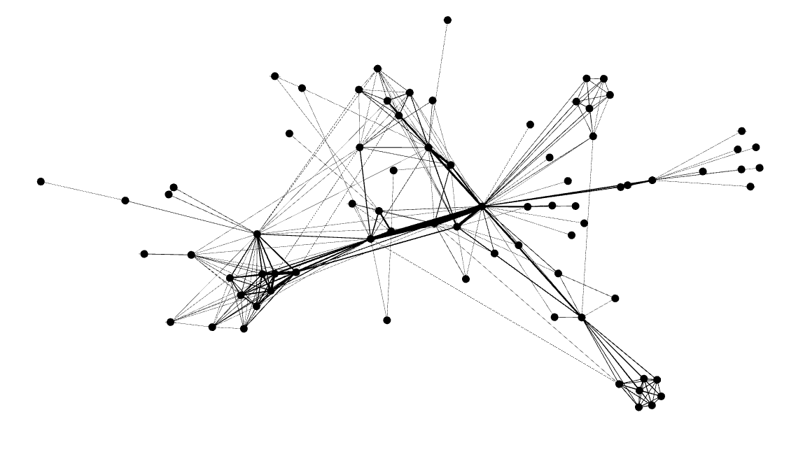
Visualizations of networks can look pretty, but of course without a formal mathematical language to describe the properties of these networks, we will not be able to quantitatively answer the questions we would like to have answered about such networks. Today I’ll introduce two ways of defining networks in terms of matrices – adjacency matrices and incidence matrices, which connects the ideas of network theory with those of linear algebra.
Adjacency Matrices
Suppose ![]() is a simple network where
is a simple network where ![]() .
.
For ![]() define
define
![Rendered by QuickLaTeX.com \[a_{ij}=\left\{\begin{aligned} 1, & \quad (i,j)\in E, \\ 0, &\quad (i,j)\not\in E.\end{aligned}\right.\]](https://genedan.com/wp-content/ql-cache/quicklatex.com-df48c868c6da5459a44c063a94cf8a48_l3.png)
Then the square matrix ![]() is called the adjacency matrix of
is called the adjacency matrix of ![]() .
.
Adjacency matrices are a way to define networks from the perspective of their nodes. The notation above simply specifies a square matrix whose rows and columns correspond to the nodes of the network. The each entry will be 1 if there is an edge connecting its corresponding row and column (which represent nodes) and 0 otherwise.
Going back to our Les Miserables example, the graph below:
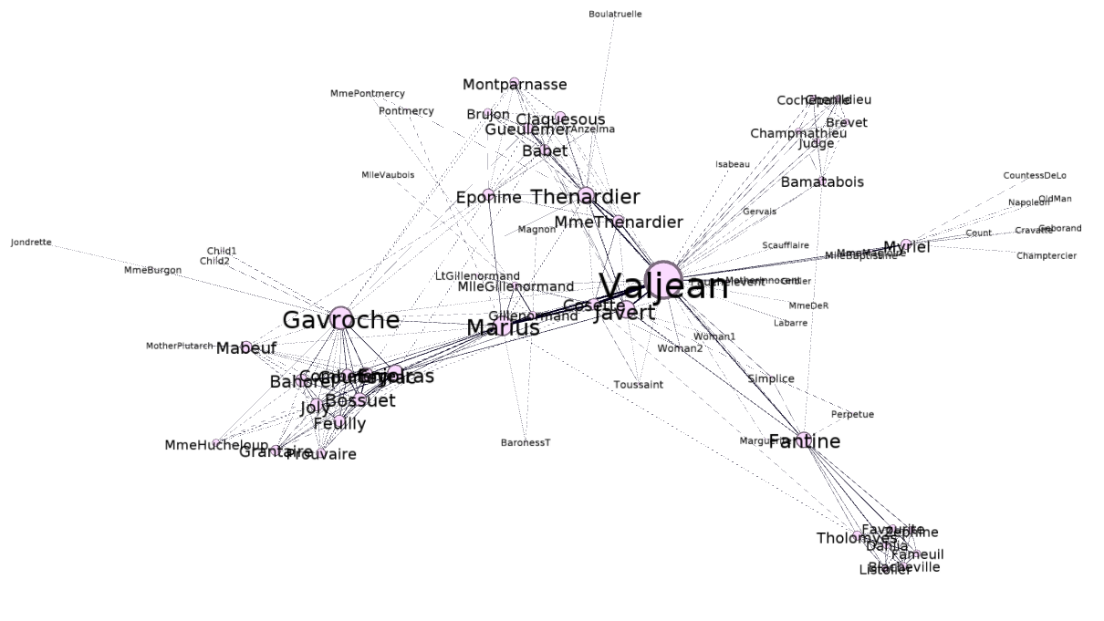
Is represented by the following adjacency matrix:
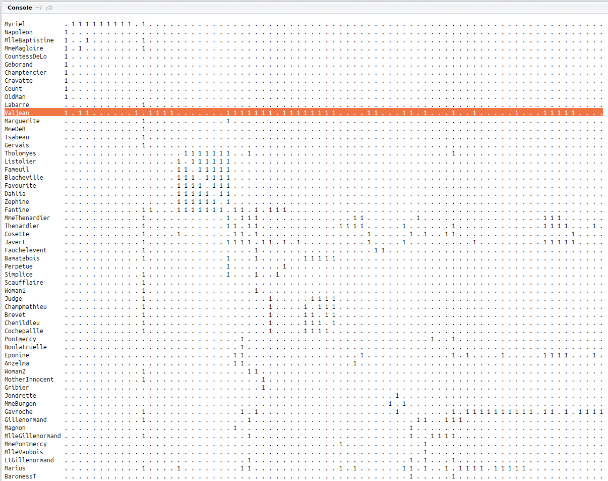
Here, the column names are omitted, but they should follow the same order as the row names. If you add up the 1s in a row, the sum should be equal to the degree of the node that it represents. For example, the sum of the row that represents Jean Valjean (highlighted in the matrix above) equals 36. This is both consistent with the data from gephi and the theory represented in the text:
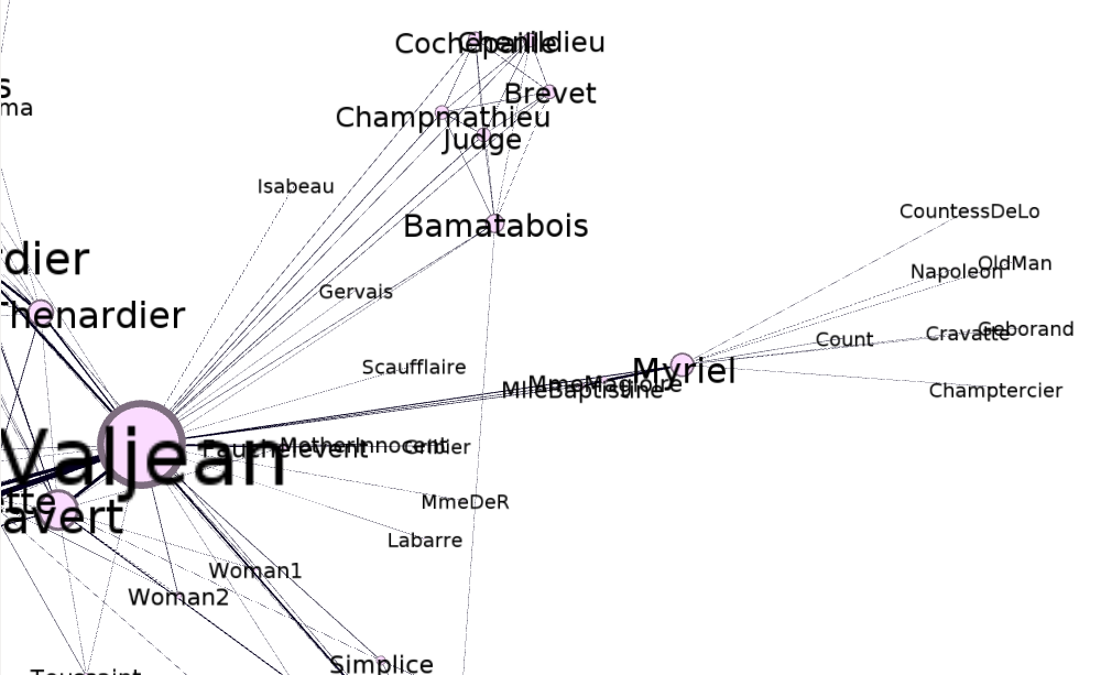
Furthermore, we can see that certain characters who are connected with Myriel have a degree of 1, such as Napoleon, Cravatte, and Champtercier, which are seen in both the matrix and the visual representation of the graph if we zoom in:
A short script was used to import the gexf data, convert it into an igraph object, and from there calculate and print the adjacency matrix.
|
1 2 3 4 5 6 7 8 9 10 11 12 13 14 15 |
library(rgexf) library(igraph) #Set options to be able to see the entire matrix options(max.print= 10000, width = 10000) #Import gexf file and convert to igraph object LesMis_gexf <- read.gexf("LesMiserables.gexf") LesMis_igraph <- gexf.to.igraph(LesMis_gexf) #Create the adjacency matrix from the data LesMis_adj <- as_adj(LesMis_igraph) #Print the adjacency matrix LesMis_adj |
Incidence Matrices
Suppose ![]() is a network where
is a network where ![]() and
and ![]() with
with ![]() .
.
For ![]() and
and ![]() define
define
![Rendered by QuickLaTeX.com \[b_{ij}=\left\{\begin{aligned} 1, & \quad u_i=j, \\ 1, &\quad v_i = j, \\ 0 & \quad \text{otherwise.}\end{aligned}\right.\]](https://genedan.com/wp-content/ql-cache/quicklatex.com-911e8bc822b2182b37287f287eafeb7e_l3.png)
Then the rectangular matrix ![]() is called the incidence matrix of
is called the incidence matrix of ![]() .
.
Incidence matrices are a way to define networks from the perspective of edges. The notation above simply means that this time, we’ll have a matrix whose columns represent each edge in the network, and the rows represent nodes. Each entry will be a 1 if the character represented by a row participates in the edge represented by the column, and zero otherwise.
Unfortunately, igraph (at least to my knowledge) can’t calculate the incidence matrix for a nonbipartite graph, so I had to use a workaround I found on stackoverflow. I’ve also altered the in the definition from the original text to be consistent with this workaround (the original had a -1 for the v’s).
The LesMiserables network has 77 nodes and 254 edges, so we’ll have a very wide matrix that is too large to display on this webpage. However, I’ve added a screenshot to give just a glimpse as to what it looks like:

The code used to generate the matrix:
|
1 2 3 |
library(intergraph) library(network) LesMis_inc <- as.matrix(asNetwork(LesMis_igraph),matrix.type="incidence") |
