• Home
  • Readings
  • Github
  • MIES
  • TmVal
  • About
Gene Dan's Blog

Monthly Archives: June 2020

You are browsing the site archives by month.

No. 140: MIES – Rate Changes – Slutsky and Hicks Decomposition

28 June, 2020 6:24 PM / Leave a Comment / Gene Dan

This entry is part of a series dedicated to MIES – a miniature insurance economic simulator. The source code for the project is available on GitHub.

Current Status

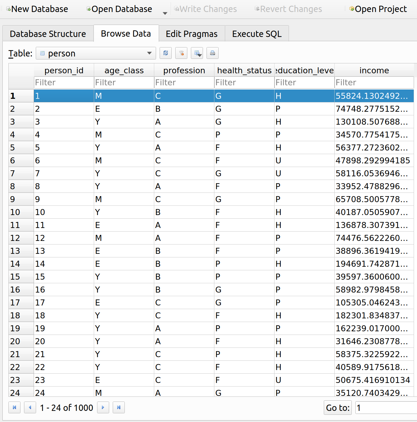
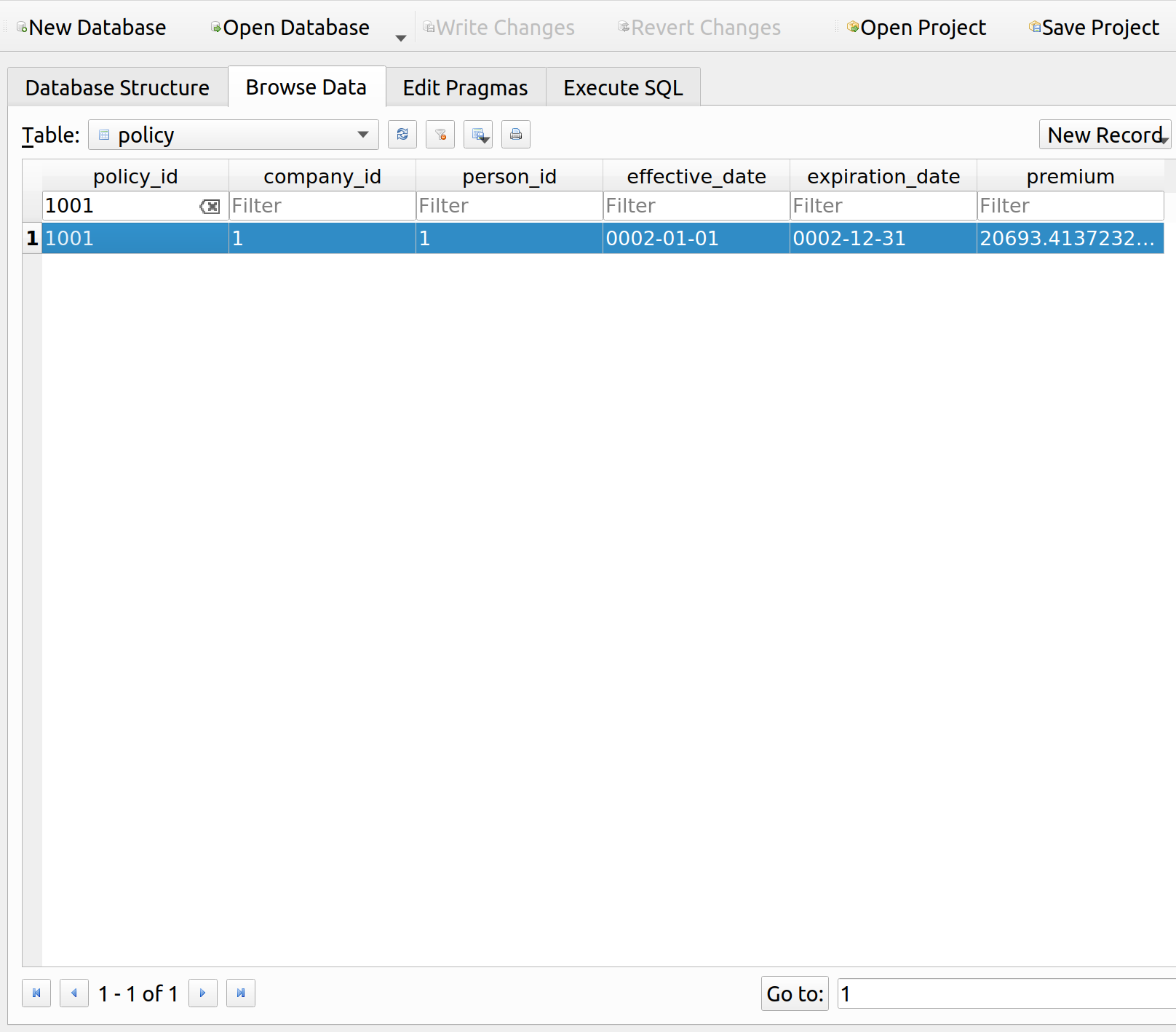
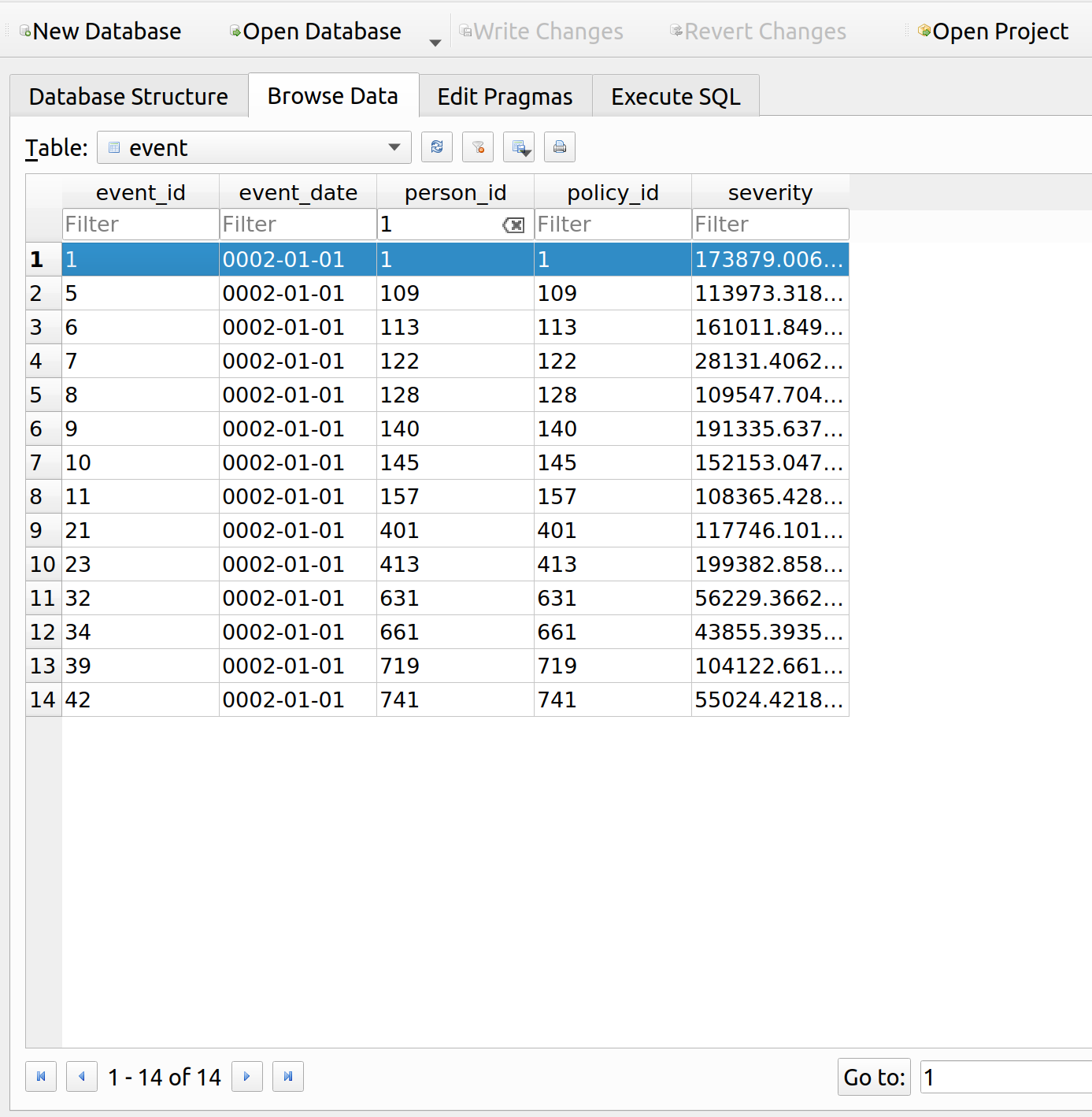
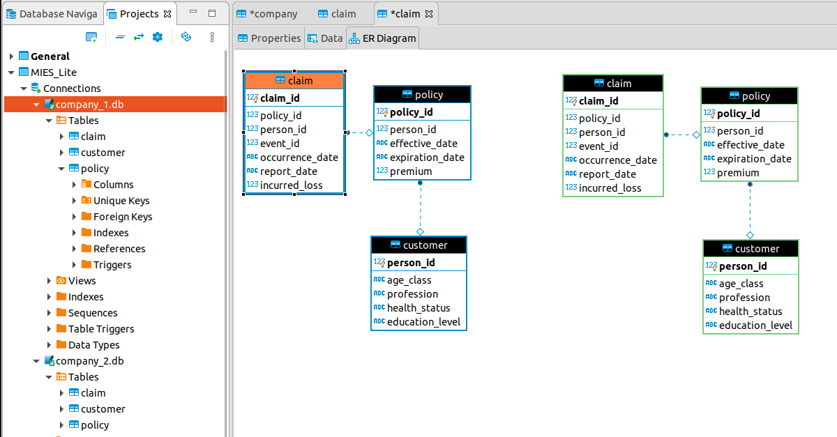
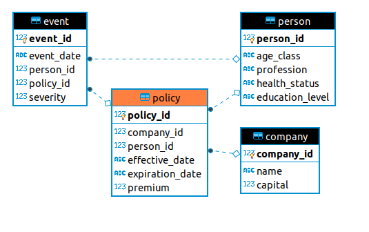
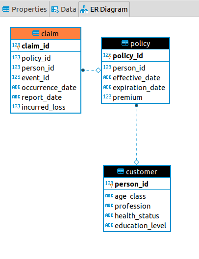
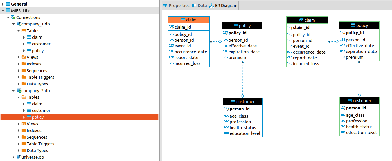
Last week, I revisited the MIES backend to split what was a single database into multiple databases – one per entity in the simulation. This enhances the level of realism and should make it easier to program transactions between the entities. This week, I’ll revisit consumer behavior by implementing the Slutsky and Hicks decomposition methods for analyzing price changes.

In the context of insurance, consumers frequently experience changes in price, typically during renewals when insurers apply updated rating algorithms against new information known about the insureds. For example, If you’ve made a claim or two during your policy period, and miss a rent payment, causing your credit score to go down, your premium is likely to increase upon renewal. This is because past claims and credit are frequently used as the underlying variables in a rating algorithm.

What happens when consumers face an increase in rates? Oftentimes, they reduce coverage, may try to shop around, or may do nothing at all and simply pay the new price. Today’s post discusses the first phenomenon, whereby an increase in rates causes a reduction in the amount of insurance that a consumer purchases. We can use the Slutsky and Hicks decomposition methods to break down this behavior into two components:

  1. The substitution effect
  2. The income effect

The substitution effect concerns the change in relative prices between two goods. Here, when a consumer faces a premium increase, the price of insurance increases relative to the price of all other goods, altering the rate at which the consumer would be willing to exchange a unit of insurance for a unit of all other goods.

The income effect concerns the change in the price of a good relative to consumer income. When a consumer faces a premium increase without a corresponding increase in income, their income affords them fewer units of insurance.

The content of this post roughly follows the content of chapter 8 in Varian. As usual, I focus on how this applies to my own project and will skip over much of the theoretical derivations that can be found in the text.

Slutsky Identity

The Slutsky identity has the following form:

    \[\frac{\Delta x_1}{\Delta p_1} = \frac{\Delta x_1^s}{\Delta p_1} - \frac{\Delta x_1^m}{\Delta m}x_1\]

Where the x_1 represents the quantity of good 1 (in this case insurance), p_1 represents the price of insurance (that is, the premium) and m represents the consumer’s income. The deltas are used to describe how the quantity of insurance purchased changes with premium, expressed on the left side of the identity. The first term after the equals sign represents the substitution effect, and the second term after the equals sign represents the income effect.

The Slutsky identity can also be expressed in terms of units instead of rates of change (\Delta x_1^m = -\Delta x_1^n):

    \[\Delta x_1 = \Delta x_1^s + \Delta x_1^n\]

While MIES can handle both forms, we’ll focus on the first form for the rest of the chapter.

Substitution Effect

Let’s examine the substitution effect. First, we’ll conduct all the steps manually, and then I’ll show how they are integrated into MIES. If we have some data already stored in a past simulation, we can extract a person from it:

Python
1
2
my_person = Person(1)
my_person.data

1
2
3
4
5
Out[12]:
   person_id age_class profession health_status education_level        income  \
0          1         E          B             F               U  89023.365436  
          wealth  cobb_c  cobb_d  
0  225300.272033     0.1     0.9  

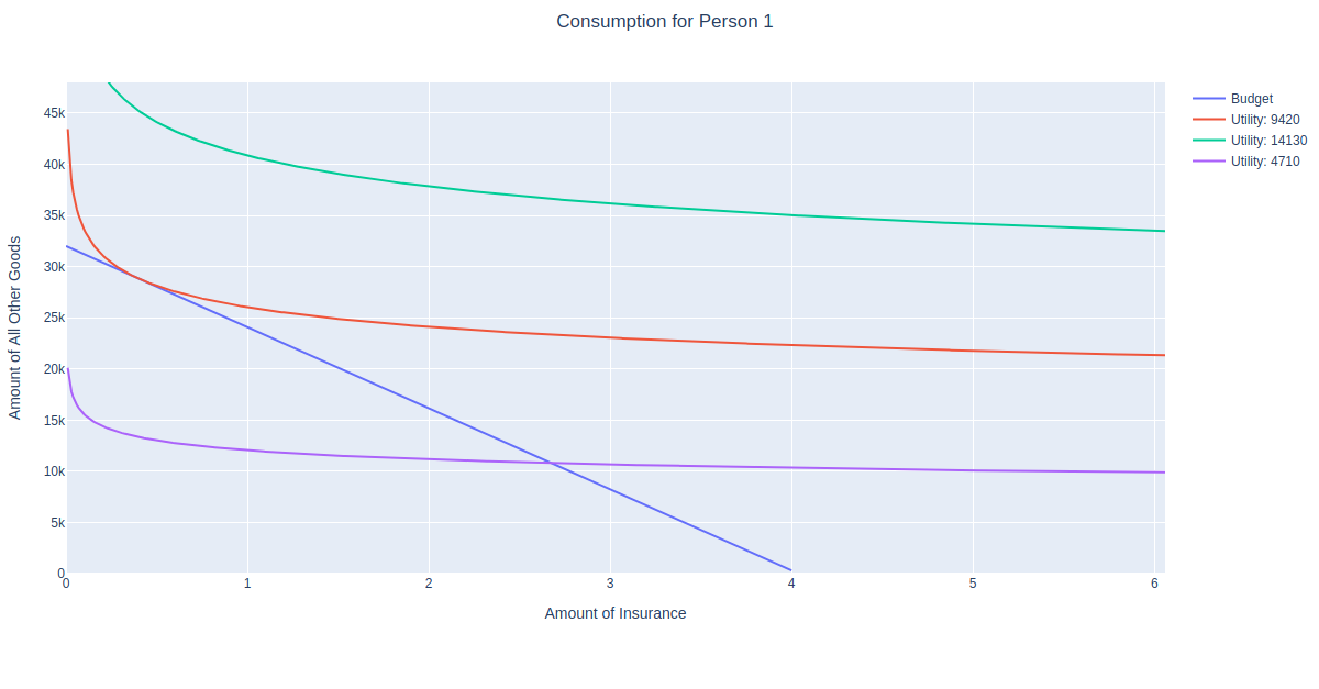
Here, we have a person who makes 89k per year, with Cobb Douglas parameters c = 0.1 and d = 0.9. This means this person will spend 10% of their income on premium. For the sake of making the graphs in this post less cluttered and easier to read, let’s change c = d = .5 so the person spends 50% of their income on insurance:

Python
1
2
3
4
5
6
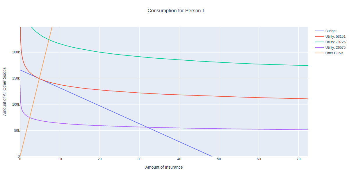
my_person.utility.c = .5
my_person.utility.d = .5
my_person.get_budget()
my_person.get_consumption()
my_person.get_consumption_figure()
my_person.show_consumption()

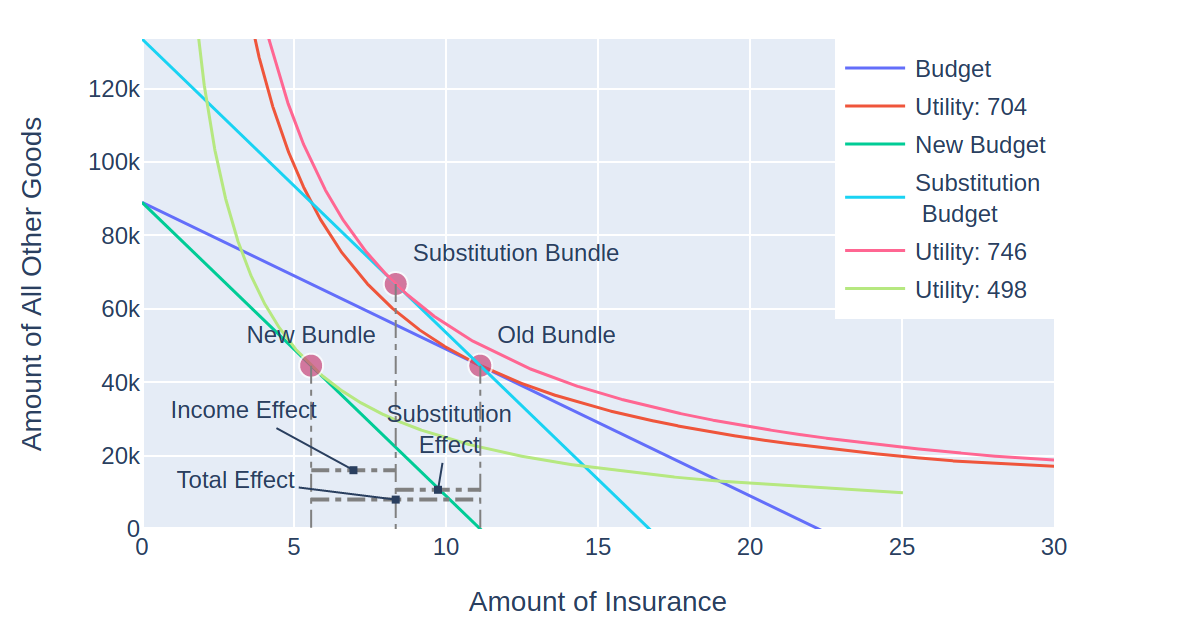
From the above figure, we can see that the person consumes about 45k worth of insurance. That’s about 11 units of exposure at a 4k premium per exposure, which is unrealistic in real life, but makes life easy for me because I haven’t bothered to update the margins of my website to accommodate wider figures. We’ll denote this bundle as ‘Old Bundle’ because we’ll compare it to the new consumption bundle after a rate change (note – if you are trying to replicate this in MIES, your figures may look a bit different, in reality I manually adjust the style of the plots so they can fit on my blog).

Now, let’s suppose the person faces a 100% increase in their rate so that their premium is 8k per unit of exposure, and construct a budget to reflect this:

Python
1
2
3
insurance = Good(8000, name='insurance')
all_other = Good(1, name='all other goods')
new_budget = Budget(insurance, all_other, income=my_person.income, name='new_budget')

Plotting this new budget, we see that the line tilts inward, since the person can only afford half as much insurance as before:

The first stage in Slutsky decomposition involves calculating the substitution effect. This is done by tilting the budget line to the slope of the new prices, but with income adjusted so that the person can still afford their old bundle. We then determine the new optimal bundle at this budget (denoted ‘substitution budget’) and call it the substitution bundle:

    \[\Delta m = x_1 \Delta p_1\]

1
2
3
sub_income = my_person.income + my_person.optimal_bundle[0] * 4000
substitution_budget = Budget(insurance, all_other, income=sub_income, name='Substitution<br /> Budget')
...more plotting code...

You can see that if the person were given enough money to purchase the same amount of insurance even after the rate increase, they would still reduce their consumption from 11.1 to 8.3 units of insurance. 8.3 – 11.1 = -2.8 is the substitution effect.

Income Effect

Now, to calculate the income effect, we then shift the substitution budget to the position of the new budget:

The person purchases 5.5 units of insurance at the new budget, so the income effect is 5.5 – 8.3 = -2.8 for the substitution effect. The total effect is -2.8 -2.8 = -5.6 units of insurance, the sum of the substitution and income effect. This is the same as the new consumption minus the old consumption 5.5 – 11.1 = -5.6

MIES Integration

The Slutsky decomposition process has been integrated into MIES as a class in econtools/slutsky.py:

Python
1
2
3
4
5
6
7
8
9
10
11
12
13
14
15
16
17
18
19
20
21
22
23
24
25
26
27
28
29
30
31
32
33
34
35
36
37
38
39
40
41
42
43
44
45
46
47
48
49
50
51
52
53
54
55
56
57
58
59
60
61
62
63
64
65
66
67
68
69
70
71
72
73
74
75
76
77
78
79
80
81
82
83
84
85
86
87
88
89
90
91
92
93
94
95
96
97
98
99
100
101
102
103
104
105
106
107
108
109
110
111
112
113
114
115
116
117
118
119
120
121
122
123
124
125
126
127
128
129
130
131
132
133
134
135
136
137
138
139
140
141
142
143
144
145
146
147
148
149
150
151
152
153
154
155
156
157
158
159
160
161
162
163
164
165
166
167
168
169
170
171
172
173
174
175
176
177
178
179
180
181
182
183
184
185
186
187
188
189
190
191
192
193
194
195
196
197
198
199
200
201
202
203
204
205
206
207
208
209
210
211
212
213
214
215
216
217
218
219
220
221
222
223
224
225
226
227
228
229
230
231
232
233
234
235
236
237
238
239
240
241
242
243
244
245
246
247
248
249
250
251
252
253
254
255
256
257
258
259
260
261
262
263
264
265
266
267
268
269
270
271
272
273
274
275
276
277
278
279
280
281
282
283
284
285
286
287
288
289
290
291
292
293
294
295
296
297
298
299
300
301
302
303
304
305
306
307
308
309
310
311
312
313
314
315
316
317
318
319
320
321
322
323
324
325
326
import plotly.graph_objects as go
 
from plotly.offline import plot
from econtools.budget import Budget
from econtools.utility import CobbDouglas
 
 
class Slutsky:
    """
    Implementation of the Slutsky equation, accepts two budgets, a utility function, and calculates
    the income and substitution effects
    """
    def __init__(
            self,
            old_budget: Budget,
            new_budget: Budget,
            utility_function: CobbDouglas  # need to replace with utility superclass
    ):
        self.old_budget = old_budget
        self.old_budget.name = 'Old Budget'
        self.new_budget = new_budget
        self.new_budget.name = 'New Budget'
        self.utility = utility_function
 
        self.old_bundle = self.utility.optimal_bundle(
            self.old_budget.good_x.price,
            self.old_budget.good_y.price,
            self.old_budget.income
        )
 
        self.delta_p = self.new_budget.good_x.price - self.old_budget.good_x.price
        self.pivoted_budget = self.calculate_pivoted_budget()
        self.substitution_bundle = self.calculate_substitution_bundle()
        self.substitution_effect = self.calculate_substitution_effect()
        self.new_bundle = self.calculate_new_bundle()
        self.income_effect = self.calculate_income_effect()
        self.total_effect = self.substitution_effect + self.income_effect
        self.substitution_rate = self.calculate_substitution_rate()
        self.income_rate = self.calculate_income_rate()
        self.slutsky_rate = self.substitution_rate - self.income_rate
        self.plot = self.get_slutsky_plot()
 
    def calculate_pivoted_budget(self):
        """
        Pivot the budget line at the new price so the consumer can still afford their old bundle
        """
        delta_m = self.old_bundle[0] * self.delta_p
        pivoted_income = self.old_budget.income + delta_m
        pivoted_budget = Budget(
            self.new_budget.good_x,
            self.old_budget.good_y,
            pivoted_income,
            'Pivoted Budget'
        )
        return pivoted_budget
 
    def calculate_substitution_bundle(self):
        """
        Return the bundle consumed after pivoting the budget line
        """
        substitution_bundle = self.utility.optimal_bundle(
            self.pivoted_budget.good_x.price,
            self.pivoted_budget.good_y.price,
            self.pivoted_budget.income
        )
        return substitution_bundle
 
    def calculate_substitution_effect(self):
        substitution_effect = self.substitution_bundle[0] - self.old_bundle[0]
        return substitution_effect
 
    def calculate_new_bundle(self):
        """
        Shift the budget line outward
        """
        new_bundle = self.utility.optimal_bundle(
            self.new_budget.good_x.price,
            self.new_budget.good_y.price,
            self.new_budget.income
        )
        return new_bundle
 
    def calculate_income_effect(self):
        income_effect = self.new_bundle[0] - self.substitution_bundle[0]
        return income_effect
 
    def calculate_substitution_rate(self):
        delta_s = self.calculate_substitution_effect()
        delta_p = self.new_budget.good_x.price - self.old_budget.good_x.price
        substitution_rate = delta_s / delta_p
        return substitution_rate
 
    def calculate_income_rate(self):
        delta_p = self.new_budget.good_x.price - self.old_budget.good_x.price
        delta_m = self.old_bundle[0] * delta_p
        delta_x1m = -self.calculate_income_effect()
        income_rate = delta_x1m / delta_m * self.old_bundle[0]
        return income_rate
 
    def get_slutsky_plot(self):
        max_x_int = max(
            self.old_budget.income / self.old_budget.good_x.price,
            self.pivoted_budget.income / self.pivoted_budget.good_x.price,
            self.new_budget.income / self.new_budget.good_x.price
        ) * 1.2
 
        max_y_int = max(
            self.old_budget.income,
            self.pivoted_budget.income,
            self.new_budget.income,
        ) * 1.2
 
        # interval boundaries
        effect_boundaries = [
            self.new_bundle[0],
            self.substitution_bundle[0],
            self.old_bundle[0]
        ]
        effect_boundaries.sort()
 
        fig = go.Figure()
 
        # budget lines
        fig.add_trace(self.old_budget.get_line())
        fig.add_trace(self.pivoted_budget.get_line())
        fig.add_trace(self.new_budget.get_line())
 
        # utility curves
        fig.add_trace(
            self.utility.trace(
                k=self.old_bundle[2],
                m=max_x_int,
                name='Old Utility'
            )
        )
        fig.add_trace(
            self.utility.trace(
                k=self.substitution_bundle[2],
                m=max_x_int,
                name='Pivoted Utility'
            )
        )
        fig.add_trace(
            self.utility.trace(
                k=self.new_bundle[2],
                m=max_x_int,
                name='New Utility'
            )
        )
        # consumption bundles
 
        fig.add_trace(
            go.Scatter(
                x=[self.old_bundle[0]],
                y=[self.old_bundle[1]],
                mode='markers+text',
                text=['Old Bundle'],
                textposition='top center',
                marker=dict(
                    size=[15],
                    color=[1]
                ),
                showlegend=False
            )
        )
 
        fig.add_trace(
            go.Scatter(
                x=[self.substitution_bundle[0]],
                y=[self.substitution_bundle[1]],
                mode='markers+text',
                text=['Pivoted Bundle'],
                textposition='top center',
                marker=dict(
                    size=[15],
                    color=[2]
                ),
                showlegend=False
            )
        )
 
        fig.add_trace(
            go.Scatter(
                x=[self.new_bundle[0]],
                y=[self.new_bundle[1]],
                mode='markers+text',
                text=['New Bundle'],
                textposition='top center',
                marker=dict(
                    size=[15],
                    color=[3]
                ),
                showlegend=False
            )
        )
        # Substitution and income effect interval lines
        fig.add_shape(
            type='line',
            x0=self.substitution_bundle[0],
            y0=self.substitution_bundle[1],
            x1=self.substitution_bundle[0],
            y1=0,
            line=dict(
                color="grey",
                dash="dashdot",
                width=1
            )
        )
 
        fig.add_shape(
            type='line',
            x0=self.new_bundle[0],
            y0=self.new_bundle[1],
            x1=self.new_bundle[0],
            y1=0,
            line=dict(
                color="grey",
                dash="dashdot",
                width=1
            )
        )
 
        fig.add_shape(
            type='line',
            x0=self.old_bundle[0],
            y0=self.old_bundle[1],
            x1=self.old_bundle[0],
            y1=0,
            line=dict(
                color="grey",
                dash="dashdot",
                width=1
            )
        )
        fig.add_shape(
            type='line',
            xref='x',
            yref='y',
            x0=effect_boundaries[0],
            y0=max_y_int / 10,
            x1=effect_boundaries[1],
            y1=max_y_int / 10,
            line=dict(
                color='grey',
                dash='dashdot'
            )
        )
        fig.add_shape(
            type='line',
            xref='x',
            yref='y',
            x0=effect_boundaries[1],
            y0=max_y_int / 15,
            x1=effect_boundaries[2],
            y1=max_y_int / 15,
            line=dict(
                color='grey',
                dash='dashdot'
            )
        )
        fig.add_shape(
            type='line',
            xref='x',
            yref='y',
            x0=effect_boundaries[0],
            y0=max_y_int / 20,
            x1=effect_boundaries[2],
            y1=max_y_int / 20,
            line=dict(
                color='grey',
                dash='dashdot'
            )
        )
 
        fig.add_annotation(
            x=(self.substitution_bundle[0] + self.old_bundle[0]) / 2,
            y=max_y_int / 10,
            text='Substitution<br />Effect',
            xref='x',
            yref='y',
            showarrow=True,
            arrowhead=7,
            ax=5,
            ay=-40,
        )
 
        fig.add_annotation(
            x=(self.new_bundle[0] + self.substitution_bundle[0]) / 2,
            y=max_y_int / 15,
            text='Income Effect',
            xref='x',
            yref='y',
            showarrow=True,
            arrowhead=7,
            ax=50,
            ay=-20
        )
 
        fig.add_annotation(
            x=(effect_boundaries[2] + effect_boundaries[0]) / 2,
            y=max_y_int / 20,
            text='Total Effect',
            xref='x',
            yref='y',
            showarrow=True,
            arrowhead=7,
            ax=100,
            ay=20
        )
 
        fig['layout'].update({
            'title': 'Slutsky Decomposition',
            'title_x': 0.5,
            'xaxis': {
                'title': 'Amount of Insurance',
                'range': [0, max_x_int]
            },
            'yaxis': {
                'title': 'Amount of All Other Goods',
                'range': [0, max_y_int]
            }
        })
        return fig
 
    def show_plot(self):
        plot(self.plot)

This has been added to the Person class, so we can use its methods to get the substitution and income effects. This conveniently packages all the manual steps we took above together:

Python
1
2
3
my_person.calculate_slutsky(new_budget)
my_person.slutsky.income_effect
my_person.slutsky.substitution_effect

Which returns -2.8 for each effect, the same as above.

Hicks Decomposition

A similar decomposition method is called Hicks decomposition. Instead of pivoting the budget constraint so that the person can afford the same bundle as before, the budget constraint is shifted so that they have the same utility as before. Using algebra, we can solve this by fixing utility:

    \[m^\prime = \frac{\bar{u}}{\left(\frac{c}{c +d}\frac{1}{p_1^\prime}\right)^c\left(\frac{d}{c+d}\frac{1}{p_2}\right)^d}\]

where m^\prime is the adjusted income, and p_1^\prime is the new premium, and \bar{u} is the utility fixed at the original level.

You’ll notice there’s a subtle difference, the new bundle is the same as in the Slutsky case, but the substitution bundle in this case is on the original utility curve. This gives different answers for the substitution and income effects, which are -3.3 and -2.3, which add up to a total effect of -5.6, as before.

The code for the Hicks class is much the same as that for the Slutsky class, so I won’t post most of it here, the relevant change is in calculating the substitution budget:

Python
1
2
3
4
5
6
7
8
9
10
11
12
13
14
15
16
17
18
19
20
21
22
23
class Hicks:
...
 
    def calculate_pivoted_budget(self):
        """
        Pivot the budget line at the new price so the consumer still as the same utility
        """
        old_utility = self.old_bundle[2]
        c = self.utility.c
        d = self.utility.d
        p1_p = self.new_budget.good_x.price
        p2 = self.old_budget.good_y.price
        x1_no_m = (((c / (c + d)) * (1 / p1_p)) ** c)
        x2_no_m = (((d / (c + d)) * (1 / p2)) ** d)
        pivoted_income = old_utility / (x1_no_m * x2_no_m)
        pivoted_budget = Budget(
            self.new_budget.good_x,
            self.old_budget.good_y,
            pivoted_income,
            'Pivoted Budget'
        )
        return pivoted_budget
        ...

Further Improvements

Since Hicks substitution is mostly similar to Slutsky in terms of code, it makes sense for the Hicks class to inherit from the Slutsky class or for both of them to inherit from a superclass.

I’m currently working on implementing wealth into MIES, since as of today, none of the transactions actually impact wealth.

Posted in: Actuarial, Mathematics, MIES / Tagged: actuarial, insurance, MIES, simulator

No. 139: MIES – Schema Changes and Claims Reporting

21 June, 2020 4:13 PM / Leave a Comment / Gene Dan

This entry is part of a series dedicated to MIES – a miniature insurance economic simulator. The source code for the project is available on GitHub.

Current Status

When programming MIES, I face a trade-off between rolling out enough features for a weekly blog post and spending more time trying to learn Python in order to code them in the most elegant way possible. If I implement things too quickly, I face the problem of accumulating bugs and technical debt, but if I spend too much time trying learn the latest libraries, I’d never get anything done. Therefore, I’ve decided to just write what I can most weeks, but revisiting the code to make it better every 3rd or 4th week, so I can implement any new technical knowledge I’d gained during that time.

Last month, I demonstrated the phenomenon of adverse selection using MIES. However, the underlying database was not a realistic depiction of the real world:

There was only one database, shared by all entities involved in the simulation – firms, people, and the environment. In business, it’s more realistic for companies to have their own internal databases, without the ability to access any other company’s database. I’ve reached point where I’ve decided that it would be difficult to add insurance operations, specifically the reporting of claims, if all entities used the same database. Therefore, I’ve decided to spend time this week setting up separate schemas for each company.

The reason why I didn’t do this earlier is because I hadn’t gone far enough in the SQLAlchemy documentation to figure out how to establish multiple metadata bases to allow each company in the simulation to access its own database. The decision I was facing last month was to either write the adverse selection demo with the knowledge I had, or to keep reading further to set things up the right way and then write about how I built nothing, but read some documentation in the hope that I’d build something later. I’d gotten tired of doing the latter one too many times, so I decided to just go for it.

This week, I was confident that I’d be able to fix the single-schema problem and add a claims reporting facility as well, so that’s what I’ll go over today.

Splitting the Database

Splitting the database involved two separate challenges:

  1. Defining the schema for each entity
  2. Rewriting the code to accept the new backend structure

This second challenge was the main motivation for updating the schema now rather than later. The more features I added to MIES, the more of them I would have to rewrite when I inevitably split the database.

First, I envisioned the database structure I wanted for each firm:

Much of this was taken from the original schema, as seen at the top of this post. The policy table contains the same information as before, minus the company id. This is because a company does not need to have this field if all of its policies belong to itself.

The customer table is new. Here, I faced the challenge of whether I wanted to maintain data integrity between the information a company knows about its own customers, and their actual attributes as they exist outside the knowledge of the firm. For example, if a person switches insurers and then changes their profession, should the original insurer know about it?

In the real world, the answer is no. This also applies to things like credit scores which can change after the company does an initial credit check. Therefore, I’ve decided to discard data integrity between companies and the environment. I may want to rethink whether I want the all-knowing environment class to at least have a canonical record of all the information in the simulation (the answer is usually yes when I write these thoughts out in a blog post).

The customer table is analogous to the person table as before, but only contains information that the firm knows about each customer. This information typically costs money to acquire when quoting policies, and is considered an underwriting expense that I will need to add later.

Lastly, I’ve added a new table for claims. I mentioned last month that since we assumed each loss was fully covered, there was no need to distinguish between losses and claims. Now that we’re facing the challenge of assigning a losses to different companies as claims, I decided to lay the groundwork now so that we can loosen this assumption when we need to. Gradually, we will see the what the differences is between a loss and a claim. A loss is a fortuitous event that happens to a person, and an insurance claim is a financial claim that a person makes against their insurer for indemnification under their policy. There is also a distinction between the loss a person endures and the loss that a company needs to pay, due to things like coverage exclusions, limits, and deductibles. The claim table will take care of many of these distinctions.

Therefore, in a two-firm simulation, we will have a database for each firm. Below, we have two ER-diagrams side-by-side for each company:

This idea carries over to the case of an n-firm simulation, where we’ll have n databases. The code that defines the firm schema now resides in a new module:

Python
1
2
3
4
5
6
7
8
9
10
11
12
13
14
15
16
17
18
19
20
21
22
23
24
25
26
27
28
29
30
31
32
33
34
35
36
37
38
39
40
41
42
43
44
45
46
47
48
49
50
51
52
53
54
55
56
57
58
59
60
61
62
63
64
65
66
67
68
69
70
71
72
73
74
75
76
77
78
79
80
81
82
83
84
85
86
87
88
89
90
91
92
93
94
95
96
97
98
99
100
101
102
103
from sqlalchemy.ext.declarative import declarative_base
from sqlalchemy import Column, Integer, Date, Float, String
from sqlalchemy import ForeignKey
from sqlalchemy.orm import relationship
 
 
Base = declarative_base()
 
 
class Customer(Base):
    __tablename__ = 'customer'
 
    person_id = Column(
        Integer,
        primary_key=True
    )
    age_class = Column(String)
    profession = Column(String)
    health_status = Column(String)
    education_level = Column(String)
 
    policy = relationship(
        "Policy",
        back_populates="customer"
    )
 
    def __repr__(self):
        return "<Customer(" \
               "age_class='%s', " \
               "profession='%s', " \
               "health_status='%s', " \
               "education_level='%s'" \
               ")>" % (
                   self.age_class,
                   self.profession,
                   self.health_status,
                   self.education_level,
               )
 
 
class Policy(Base):
    __tablename__ = 'policy'
 
    policy_id = Column(
        Integer,
        primary_key=True
    )
    person_id = Column(
        Integer,
        ForeignKey('customer.person_id')
    )
    effective_date = Column(Date)
    expiration_date = Column(Date)
    premium = Column(Float)
 
    customer = relationship(
        "Customer",
        back_populates="policy"
    )
 
    def __repr__(self):
        return "<Policy(person_id ='%s'," \
               "effective_date ='%s', " \
               "expiration_date='%s', " \
               "premium='%s')>" % (
                self.person_id,
                self.effective_date,
                self.expiration_date,
                self.premium
                )
 
 
class Claim(Base):
    __tablename__ = 'claim'
 
    claim_id = Column(
        Integer,
        primary_key=True
    )
    policy_id = Column(
        Integer,
        ForeignKey('policy.policy_id')
    )
    person_id = Column(Integer)
    event_id = Column(Integer)
    occurrence_date = Column(Date)
    report_date = Column(Date)
    incurred_loss = Column(Float)
 
    def __repr__(self):
        return "<Claim(policy_id ='%s'," \
               "person_id ='%s', " \
               "event_id='%s', " \
               "occurrence_date='%s'," \
               "report_date='%s'," \
               "incurred_loss='%s')>" % (
                self.policy_id,
                self.person_id,
                self.event_id,
                self.occurence_date,
                self.report_date,
                self.incurred_loss
                )

There is also a schema for the environment, which is similar to before but minus the policy-specific information:

Query Encapsulation

MIES relies on querying its databases to run the simulations. Up until now, many of these queries resided within the environment, broker, and insurer classes. The tricky thing about querying databases is that you should close the connections to them once you no longer need them. However, establishing and closing a database requires a few lines of code, and the queries themselves can be verbose as well. This can get repetitive and can lead to bugs if I forget to close a connection or make modifications to reused queries.

Therefore, I thought it would be a good idea to encapsulate them into functions. In order to do this, I created two modules in a folder called utilities that are used to connect to and then query the databases, respectively. For example, the connections file contains code to connect to either the universe (environment) database or the database for a particular company:

1
2
3
4
5
6
7
8
9
10
11
12
13
14
15
16
17
18
19
20
21
22
import sqlalchemy as sa
from sqlalchemy.orm import sessionmaker
import schema.universe as universe
 
 
def connect_universe():
    engine = sa.create_engine(
        'sqlite:///db/universe.db',
        echo=True
    )
    session = sessionmaker(bind=engine)()
    connection = engine.connect()
    return session, connection
 
 
def connect_company(company_name):
    engine = sa.create_engine(
        'sqlite:///db/companies/' + company_name + '.db',
        echo=True)
    session = sessionmaker(bind=engine)()
    connection = engine.connect()
    return session, connection

You can see that you need to import some things, and also define an engine, session, and connection. That’s quite a bit of code that I don’t want to repeat every time I need to access a database.

Moving onto the queries, we likewise have code that we don’t want to repeat. For example, the query_population() function in the queries file returns the PersonTable from the environment schema as a dataframe:

1
2
3
4
5
6
7
8
9
10
11
12
13
14
import pandas as pd
 
from schema.universe import Company, PersonTable
from schema.insco import Customer, Policy
from utilities.connections import (
    connect_universe,
    connect_company)
 
def query_population():
    session, connection = connect_universe()
    query = session.query(PersonTable).statement
    population = pd.read_sql(query, connection)
    connection.close()
    return population

Now, rather than calling all the code that we see within these functions, we can just get the information in one line, that is, query_population(). Other queries within the file access other parts of the database and return information we might want to ask about frequently:

Python
1
2
3
4
5
6
7
8
9
10
11
12
13
14
15
16
17
18
19
20
21
22
23
24
25
26
27
28
29
30
31
32
33
34
35
36
37
38
39
40
41
42
43
44
45
46
47
48
49
50
51
52
53
54
55
56
57
58
59
60
61
62
63
64
65
66
67
68
69
70
71
72
73
74
75
76
77
78
79
80
81
82
83
84
85
86
87
88
89
def query_company():
    session, connection = connect_universe()
    companies_query = session.query(Company).statement
    companies = pd.read_sql(
        companies_query,
        connection
    )
    connection.close()
    return companies
 
 
def query_all_policies():
    companies = query_company()
    policies = pd.DataFrame()
 
    for index, row in companies.iterrows():
        company_id = row['company_id']
        company_name = row['company_name']
        session, connection = connect_company(company_name)
        query = session.query(Policy).statement
        policy_c = pd.read_sql(
            query,
            connection
        )
        policy_c['company_id'] = company_id
        policy_c['company_name'] = company_name
        policies = policies.append(policy_c)
        connection.close()
 
    return policies
 
 
def query_in_force_policies(curr_date):
    companies = get_company_names()
    in_force = pd.DataFrame()
 
    for company in companies:
        session, connection = connect_company(company)
 
        exp_query = session.query(
            Policy
        ).filter(
            Policy.expiration_date == curr_date
        ).statement
 
        company_in_force = pd.read_sql(
            exp_query,
            connection)
 
        in_force = in_force.append(
            company_in_force,
            ignore_index=True
        )
 
        connection.close()
    return in_force
 
 
def get_company_names():
    session, connection = connect_universe()
    companies_query = session.query(Company.company_name).statement
    companies = pd.read_sql(
        companies_query,
        connection
    )
    connection.close()
    return list(companies['company_name'])
 
 
def get_company_ids():
    session, connection = connect_universe()
    companies_query = session.query(Company.company_id).statement
    companies = pd.read_sql(companies_query, connection)
    connection.close()
    return list(companies['company_id'])
 
 
def get_uninsured_ids(curr_date):
    population = query_population()
    in_force = query_in_force_policies(curr_date)
    uninsureds = population[~population['person_id'].isin(in_force['person_id'])]['person_id']
    return uninsureds
 
 
def get_customer_ids(company):
    session, connection = connect_company(company)
    id_query = session.query(Customer.person_id).statement
    ids = pd.read_sql(id_query, connection)
    return ids

Claims Reporting

If you looked carefully, you may have noticed an additional date field added since last month. In addition to the event date, synonymous with occurrence date, we now have the report date – that is, the date the claim is reported to the insurer. This distinction has important implications in actuarial science, since different types of policies exist that may only offer coverage on claims that either occur during or are reported during the period the policy is in effect.

For now, I have assumed that all policies are written on an occurrence basis, which means that a policy covers all claims that occur within the coverage period. This means that even if an insured reports a claim several years after is has occurred and can prove that its valid and occurred during the policy period, it is still covered under the terms of the policy.

I decided to add the claims reporting facility as a method in the broker class, which now resembles more of a place where transactions happen than an actual brokerage:

Python
1
2
3
4
5
6
7
8
9
10
11
12
13
14
15
16
17
18
19
20
21
22
23
24
25
26
27
28
29
30
31
32
33
34
35
36
37
38
39
40
41
42
43
44
45
46
47
48
    def report_claims(self, report_date):
        # match events to policies in which they are covered
        session, connection = connect_universe()
 
        event_query = session.query(Event).\
            filter(Event.report_date == report_date).\
            statement
 
        events = pd.read_sql(event_query, connection)
        connection.close()
 
        policies = query_all_policies()
        claims = events.merge(
            policies,
            on='person_id',
            how='left'
        )
        claims = claims.query(
            'event_date >= effective_date '
            'and event_date <= expiration_date'
        )
 
        claims = claims.drop([
            'effective_date',
            'expiration_date',
            'premium',
            'company_id'
        ], axis=1)
 
        companies = get_company_names()
        for company in companies:
            reported_claims = claims[claims['company_name'] == company]
 
            reported_claims = reported_claims.rename(columns={
                'event_date': 'occurrence_date',
                'ground_up_loss': 'incurred_loss'
            })
 
            reported_claims = reported_claims.drop(['company_name'], axis=1)
 
            session, connection = connect_company(company)
            reported_claims.to_sql(
                'claim',
                connection,
                index=False,
                if_exists='append'
            )
            connection.close()

This function takes the report date as an argument, and then combs through both the event table from the environment and the policy table from each company to match the event to the appropriate company and policy, and then populate that company’s claim table.

The actual claims cycle is much more complex, involving adjusters, claimants, lawyers, agents, and other parties. These have been abstracted away for now, but I plan to add more detail later since claims modeling is itself an important part of an insurer’s strategy.

I’ve also made many changes to the other classes, but I wanted to highlight claims reporting since it’s a new feature. You can examine the other changes on GitHub.

Simulation

By encapsulating the queries, I’ve removed the number of arguments and lines of code needed to run the simulations. For example, we can now define an Insurer with just two arguments:

Python
1
2
3
company_1 = Insurer(4000000, 'company_1')
 
company_2 = Insurer(4000000, 'company_2')

Whereas previously, it took five aguments:

Python
1
2
3
company_1 = Insurer(gsession, engine, 4000000, Company, 'company_1')
 
company_2 = Insurer(gsession, engine, 4000000, Company, 'company_2')

The need to specify the connection, engine, and table was cumbersome and is now handled automatically by the Insurer class.

Finally, I tested out how the data flows from policy issuance to claims occurrence, and then to renewals, and MIES is still able to demonstrate the phenomenon of adverse selection:

Further Improvements

I’d like to get back to the subject of economics next week, so now I’m working on implementing the Slutsky Equation, which decomposes the motivations a consumer might have for changing their consumption as prices change.

Posted in: Actuarial, Mathematics, MIES

No. 138: MIES – Offer, Engel, and Personal Demand Curves

14 June, 2020 10:11 PM / Leave a Comment / Gene Dan


This entry is part of a series dedicated to MIES – a miniature insurance economic simulator. The source code for the project is available on GitHub.

Current Status

Last week, I specified a Cobb Douglas utility curve for each person in MIES. I also demonstrated a situation in which a person might choose to not fully insure. However, I’ve gone a few chapters ahead in my readings and found out that under certain assumptions, a risk-averse person who is offered a fair premium will choose to fully insure. In MIES, since each company charges the pure premium without loading for profit or expenses, each person is getting a fair premium – so there’s something missing from my current model that makes it inconsistent with economic theory.

Risk aversion is not yet implemented in MIES, and will have to wait a few weeks before I get to it, since there’s quite a bit of work to do. But I’m mentioning the issue here, just in case someone reading this knows more about the subject than I do.

This week, I’m going to demonstrate a set of tools to examine consumer choice – the offer, Engel, and personal demand curves. I don’t recall using the first two curves very much in my economics courses, but the latter will be very important and will serve as a bridge between personal demand and market demand. Surprisingly, these curves were very quick to implement, since they all rely on the same method I wrote last week for the Cobb Douglas class.

The topic of this post roughly corresponds to chapter 6 of Varian.

Offer Curve

The offer curve for a consumer depicts their optimal consumption bundle at each level of income. Since the offer curve is unique to a particular consumer, I decided to define the methods that generate and plot the offer curve within the Person class. Luckily, the CobbDouglas class that I defined last week has a method called optimal_bundle, which returns the optimal consumption bundle given a set of prices and income. Since this is exactly what we need given the definition of the offer curve, we can simply use this method to generate each person’s offer curve:

Python
1
2
3
4
5
6
7
8
9
10
    def get_offer(self):
        # only works for Cobb Douglas right now
        def o(m):
            return self.utility.optimal_bundle(
                p1=self.premium,
                p2=1,
                m=m
            )
 
        self.offer = o

Note that while I only have one utility curve defined in MIES at the moment (Cobb Douglas), the definition of the offer curve doesn’t need to have anything specific to the Cobb Douglas utility function. This means in the future, I should be able to abstract this method to accept other utility functions without too much modification.

I’ve also added a method to plot a person’s offer curve:

Python
1
2
3
4
5
6
7
8
9
10
11
12
13
14
15
    def show_offer(self):
        offer_frame = pd.DataFrame(columns=['income'])
        offer_frame['income'] = np.arange(0, self.income * 2, 1000)
        offer_frame['x1'], offer_frame['x2'] = self.offer(offer_frame['income'])[:2]
 
        offer_trace = {
            'x': offer_frame['x1'],
            'y': offer_frame['x2'],
            'mode': 'lines',
            'name': 'Offer Curve'
        }
 
        fig = self.consumption_figure
        fig.add_trace(offer_trace)
        plot(fig)

This method takes a preset range of income values, and uses the get_offer method to plot the optimal consumption bundle for each income value in the range. For example if we’ve already run a few iterations of a market simulation, we can examine what combinations of insurance and non-insurance a person can afford at different income levels. Let’s do this for the person with id=1:

1
2
3
4
5
6
7
8
my_person = Person(session=gsession, engine=engine, person=PersonTable, person_id=1)
my_person.get_policy(Policy, 1001)
 
my_person.get_budget()
my_person.get_consumption()
my_person.get_consumption_figure()
my_person.get_offer()
my_person.show_offer()

Imagine what would happen if you were to shift the blue budget line inward and outward. The optimal consumption bundle would the the point of tangency with the corresponding utility function. We can see that the orange offer curve is the set of all these points.

Engel Curve

The Engel curve is similar to the offer curve, but plots the optimal choice of a good at various levels of income. Its definition within the Person class is also similar, except we only need to return the first good of the optimal bundle:

Python
1
2
3
4
5
6
7
8
9
10
11
    def get_engel(self):
        # only works for Cobb Douglas right now
 
        def e(m):
            return self.utility.optimal_bundle(
                p1=self.premium,
                p2=1,
                m=m
            )[0]
 
        self.engel = e

1
2
3
4
5
6
7
8
9
10
11
12
13
14
15
16
17
18
19
20
21
22
23
24
25
26
27
    def show_engel(self):
        engel_frame = pd.DataFrame(columns=['income'])
        engel_frame['income'] = np.arange(0, self.income * 2, 1000)
        engel_frame['x1'] = engel_frame['income'].apply(self.engel)
 
        engel_trace = {
            'x': engel_frame['x1'],
            'y': engel_frame['income'],
            'mode': 'lines',
            'name': 'Engel Curve'
        }
 
        fig = go.Figure()
        fig.add_trace(engel_trace)
 
        fig['layout'].update({
            'title': 'Engel Curve for Person ' + str(self.id),
            'title_x': 0.5,
            'xaxis': {
                'title': 'Amount of Insurance'
            },
            'yaxis': {
                'title': 'Income'
            }
        })
 
        plot(fig)

Let’s see what the Engel curve looks like for person 1:

1
2
3
4
5
6
7
8
9
my_person = Person(session=gsession, engine=engine, person=PersonTable, person_id=1)
my_person.get_policy(Policy, 1001)
my_person.premium
my_person.get_budget()
my_person.get_consumption()
my_person.get_consumption_figure()
 
my_person.get_engel()
my_person.show_engel()

Demand Curve

The demand function depicts how much of a good a person would buy if it were at a certain price. This one’s important since we’ll need it to derive industry demand, which will then be used to answer many fundamental questions about the insurance market. Like the other curves, defining this one was simple, we just get the optimal bundle at each price and return the quantity demanded of the first good:

Python
1
2
3
4
5
6
7
8
9
10
11
    def get_demand(self):
        # only works for Cobb Douglas right now
 
        def d(p):
            return self.utility.optimal_bundle(
                p1=p,
                p2=1,
                m=self.income
            )[0]
 
        self.demand = d

Python
1
2
3
4
5
6
7
8
9
10
11
12
13
14
15
16
17
18
19
20
21
22
23
24
25
26
27
28
    def show_demand(self):
        demand_frame = pd.DataFrame(columns=['price'])
        demand_frame['price'] = np.arange(self.premium/100, self.premium * 2, self.premium/100)
        demand_frame['x1'] = demand_frame['price'].apply(self.demand)
 
        demand_trace = {
            'x': demand_frame['x1'],
            'y': demand_frame['price'],
            'mode': 'lines',
            'name': 'Demand Curve'
        }
 
        fig = go.Figure()
        fig.add_trace(demand_trace)
 
        fig['layout'].update({
            'title': 'Demand Curve for Person ' + str(self.id),
            'title_x': 0.5,
            'xaxis': {
                'range': [0, self.income / self.premium * 2],
                'title': 'Amount of Insurance'
            },
            'yaxis': {
                'title': 'Premium'
            }
        })
 
        plot(fig)

Let’s see what the demand curve looks like for person 1:

1
2
3
4
5
6
7
8
9
10
my_person = Person(session=gsession, engine=engine, person=PersonTable, person_id=1)
my_person.get_policy(Policy, 1001)
my_person.premium
my_person.get_budget()
my_person.get_consumption()
my_person.get_consumption_figure()
my_person.get_offer()
 
my_person.get_demand()
my_person.show_demand()

Note that the demand curve slopes downward as it should, since we’d expect a person to buy more insurance the cheaper it is. However, note that there is no price such that the demand equals zero. The demand curve asymptotically approaches zero as the premium increases, but this particular person will never go uninsured. This is due the property of the Cobb Douglas utility function that the exponent of the good equals the percent of income spent on that good, which is hard coded as 10% at the moment. However, in the real world people do go uninsured, and this is a subject of great interest to me, so we’ll need to revisit this later.

Further Improvements

I’ve added quite a few features to the person class, but I haven’t integrated them to the point where I can perform more than two market simulations. I’m also several chapters ahead in my readings than what I’ve posted about, and I’ve encountered an interesting demonstration on risk aversion and intertemporal choice concerning assets, which will take quite an effort to both implement and reconcile with what I’ve written so far.

Posted in: Actuarial, Mathematics, MIES

No. 137: MIES – Cobb-Douglas Utility

7 June, 2020 3:30 PM / Leave a Comment / Gene Dan


This entry is part of a series dedicated to MIES – a miniature insurance economic simulator. The source code for the project is available on GitHub.

Current Status

Last week, I demonstrated how MIES can be used to calculate the budget constraint for each insured in the marketplace. This answered the question – how much insurance can each person afford during each underwriting period?

Although we now have the set of all possible consumption bundles that each person can afford, we still have no method for determining what bundle they will ultimately select – that is, how much insurance will each person actually buy? To answer this question, we turn to the concept of utility. Utility is a measurement of the satisfaction a person receives from a course of action, and we will assume that rational people seek to maximize their utility under scarcity. In this case, the course of action is purchasing insurance, and people seek to maximize their utility subject to the constraint of what they can afford.

Thus, for today’s post I will demonstrate how MIES can assign a utility function to each person in the market and determine each how much insurance each person will purchase.

By introducing utility, I would eventually like to answer certain questions I had about the insurance industry when I thought about building MIES. None of these will be answered today, but this should take us one step closer:

  1. How much insurance will be purchased in total at market equilibrium?
  2. Who will go uninsured?
  3. Should there be a mandatory minimum amount of insurance required by law? If so, should there be a state-run high-risk pool? And if so, how should it be funded?

More detailed treatment of utility can be found in chapters 4 and 5 of Varian.

Utility

To model each person’s preferences for insurance consumption, I’ve decided to use the Cobb-Douglas utility function:

    \[u(x_1, x_2) = x_1^c x_2^d\]

Where c and d represent the percentage of income spent on goods x_1 and x_2 when c + d = 1, and each x represents the quantity of each good. While other utility functions may eventually prove to be more realistic for our simulation, Cobb-Douglas utility functions are a good candidate to start with since they have many convenient features. For example, in order to find the optimal consumption bundle for a person, we need to find the bundle of goods such that the marginal rate of substitution (MRS) equals the slope of the budget constraint, while satisfying the budget constraint itself. For the Cobb-Douglas utility function, Varian provides a derivation for the MRS:

    \[\text{MRS} = -\frac{\partial u(x_1, x_2) / \partial x_1}{\partial u(x_1, x_2) / \partial x_2} \]

This can then be used with the budget constraint, p_1 x_1 + p_2 x_2 = m, to solve for the quantities of x_1 and x_2 given the income and price of each good:

    \[x_1 = \frac{c}{c + d}\frac{m}{p_1}\]

    \[x_2 = \frac{d}{c + d} \frac{m}{p_2}\]

and, when c + d = 1, x_1 = cm / p_1 and x_2 = dm/p_2. This means that using this result, we can find the optimal consumption bundle algebraically. This is very useful since 1) I have simply forgotten a lot of calculus since leaving school and 2) I won’t have to program calculus into MIES for the time being.

The convexity of the Cobb-Douglas utility function also satisfies certain assumptions underlying consumer behavior. Chapter 3 of Varian provides an in-depth explanation of these assumptions.

Utility Module

I hinted last week that I thought it might be a good idea to break up the econtools.py module into more specific modules. I’ve decided to do this to improve readability and to keep things organized. I’ve created a new folder called econtools to house these modules. The Budget class is now in the budget.py module and the utility function classes are now in a file called utility.py.

The utility.py module contains a single class, called CobbDouglas:

Python
1
2
3
4
5
6
7
8
9
10
11
12
13
14
15
16
17
18
19
20
21
22
23
24
25
26
27
28
29
30
31
32
33
34
35
36
37
38
39
40
41
42
43
44
45
46
47
import plotly.graph_objects as go
import numpy as np
 
from plotly.offline import plot
 
 
class CobbDouglas:
 
    def __init__(self, c, d):
        self.c = c
        self.d = d
 
    def optimal_bundle(self, p1, p2, m):
        x1_quantity = (self.c / (self.c + self.d)) * (m / p1)
        x2_quantity = (self.d / (self.c + self.d)) * (m / p2)
 
        optimal_utility = (x1_quantity ** self.c) * (x2_quantity ** self.d)
 
        return x1_quantity, x2_quantity, optimal_utility
 
    def trace(self, k, m):
        x_values = np.arange(.01, m * 1.5,.01)
        y_values = (k/(x_values ** self.c)) ** (1/self.d)
 
        return {'x': x_values,
                'y': y_values,
                'mode': 'lines',
                'name': 'Utility: ' + str(int(round(k)))}
 
    def show_plot(self, k=5, m=10):
        fig = go.Figure(data=self.trace(k, m))
        fig.add_trace(self.trace(k * 1.5, m))
        fig.add_trace(self.trace(k * .5, m))
        fig['layout'].update({
            'title': 'Cobb Douglas Utility',
            'title_x': 0.5,
            'xaxis': {
                'range': [0, m * 1.5],
                'title': 'Amount of Good X'
            },
            'yaxis': {
                'range': [0, m * 1.5],
                'title': 'Amount of Good Y'
            },
            'showlegend': True
        })
        plot(fig)

The CobbDouglas class takes two arguments, c and d, which correspond to the c and d parameters in the function definition. The class provides three methods: optimal_bundle() calculates the optimal consumption bundle using the results derived by Varian, trace() defines the curve as it will appear when plotted, and show_plot() plots the utility function.

Here’s an example on how to use the class to plot the function:

Python
1
2
3
4
from econtools import CobbDouglas
 
corn_on_the_cobb = CobbDouglas(.5, .5)
corn_on_the_cobb.show_plot()

Here, we’ve provided a simple example where c = d = .5, which means that the consumer will allocate 50% of their income to each good. If the price of each good is the same, the line connecting all optimal consumption bundles will go through the origin (more on that for a later post).

MIES Integration

The Person Class

Now that we’ve got a class defined for our Cobb Douglas function, we now need to find a way to get it working with MIES. I’d like to be able to access the utility function for each consumer in the simulation. Since I’ve started to examine more person-specific characteristics, I’ve created a new class in the entities.py module, Person:

Python
1
2
3
4
5
6
7
8
9
10
11
12
13
14
15
16
17
18
19
20
21
22
23
24
25
26
27
28
29
30
31
32
33
34
35
36
37
38
39
40
41
42
43
44
45
46
47
48
49
50
51
52
53
54
55
56
57
58
59
60
61
62
63
64
65
66
67
68
69
70
71
72
73
74
75
76
77
78
79
80
81
82
83
84
85
86
87
88
class Person:
    def __init__(
        self,
        session,
        engine,
        person,
        person_id
    ):
        self.session = session
        self.connection = engine.connect()
        self.engine = engine
        self.id = person_id
 
        query = self.session.query(person).filter(
                person.person_id == int(self.id)
            ).statement
 
        self.data = pd.read_sql(
            query,
            self.connection
        )
        self.income = self.data['income'].loc[0]
 
        self.utility = CobbDouglas(
            c=self.data['cobb_c'].loc[0],
            d=self.data['cobb_d'].loc[0]
        )
 
        self.policy = None
        self.budget = None
        self.premium = None
        self.optimal_bundle = None
        self.consumption_figure = None
 
    def get_policy(
        self,
        policy,
        policy_id
    ):
        query = self.session.query(policy).filter(
            policy.policy_id == int(policy_id)
        ).statement
 
        self.policy = pd.read_sql(
            query,
            self.connection
        )
        self.premium = self.policy['premium'].loc[0]
 
    def get_budget(self):
        all_other = Good(1, name='All Other Goods')
        if self.policy is None:
            insurance = Good(4000, name='Insurance')
        else:
            insurance = Good(self.premium, name='Insurance')
        self.budget = Budget(insurance, all_other, income=self.income, name='Budget')
 
    def get_consumption(self):
        self.optimal_bundle = self.utility.optimal_bundle(
            p1=self.premium,
            p2=1,
            m=self.income
        )
 
    def get_consumption_figure(self):
        fig = go.Figure()
        fig.add_trace(self.budget.get_line())
        fig.add_trace(self.utility.trace(k=self.optimal_bundle[2], m=self.income / self.premium * 1.5))
        fig.add_trace(self.utility.trace(k=self.optimal_bundle[2] * 1.5, m=self.income / self.premium * 1.5))
        fig.add_trace(self.utility.trace(k=self.optimal_bundle[2] * .5, m=self.income / self.premium * 1.5))
 
        fig['layout'].update({
            'title': 'Consumption for Person ' + str(self.id),
            'title_x': 0.5,
            'xaxis': {
                'title': 'Amount of Insurance',
                'range': [0, self.income / self.premium * 1.5]
            },
            'yaxis': {
                'title': 'Amount of All Other Goods',
                'range': [0, self.income * 1.5]
            }
        })
        self.consumption_figure = fig
        return fig
 
    def show_consumption(self):
        plot(self.consumption_figure)

Since there is already a Person class in the schema.py module referencing a SQLite table, I’ve renamed that class to PersonTable. The Person class takes a database connection, along with the person table in the database, queries the details of a person, and generates a utility function for that person. The Person class provides additional methods for attaching policy information, calculating that person’s budget, and determining how much insurance they will buy.

To keep things simple, I’ve assumed that each person’s c parameter equals, .1, which means that the population has homogeneous preferences for insurance, and will spend 10% of their income on it. The parameters.py module and environment class have been updated accordingly to reflect this. We can loosen these assumptions later on.

Optimal Consumption

Let’s find one person’s optimal bundle for purchasing insurance. To do this, we run two iterations of the simulation and examine the results for person_id = 1, like we did last week:

Python
1
2
3
4
5
6
7
8
9
10
11
12
13
14
15
16
17
18
19
20
21
22
23
24
25
26
27
28
29
30
31
32
33
34
35
36
37
38
39
40
41
import pandas as pd
import datetime as dt
import sqlalchemy as sa
import econtools as ec
from SQLite.schema import PersonTable, Policy, Base, Company, Event
from sqlalchemy.orm import sessionmaker
from entities import God, Broker, Insurer, Person
import numpy as np
import plotly.graph_objects as go
from plotly.offline import plot
 
 
pd.set_option('display.max_columns', None)
 
 
engine = sa.create_engine('sqlite:///MIES_Lite.db', echo=True)
Session = sessionmaker(bind=engine)
Base.metadata.create_all(engine)
 
gsession = Session()
 
 
ahura = God(gsession, engine)
ahura.make_population(1000)
 
pricing_date = dt.date(1, 12, 31)
 
 
rayon = Broker(gsession, engine)
company_1 = Insurer(gsession, engine, 4000000, Company, 'company_1')
company_1_formula = 'severity ~ age_class + profession + health_status + education_level'
pricing_status = 'initial_pricing'
free_business = rayon.identify_free_business(PersonTable, Policy, pricing_date)
 
companies = pd.read_sql(gsession.query(Company).statement, engine.connect())
 
rayon.place_business(free_business, companies, pricing_status, pricing_date, company_1)
ahura.smite(PersonTable, Policy, pricing_date + dt.timedelta(days=1))
company_1.price_book(PersonTable, Policy, Event, company_1_formula)
pricing_status = 'renewal_pricing'
rayon.place_business(free_business, companies, pricing_status, pricing_date, company_1)

This person has an income of about 32k. You can also see additional columns for their Cobb Douglas parameters. If all goes well, we would expect them to want to spend about 3200 on insurance. Let’s query their renewal quote to see how much premium they need to pay:

Python
1
2
my_person = Person(session=gsession, engine=engine, person=PersonTable, person_id=1)
my_person.get_policy(Policy, 1001)

Since their premium is about 8k, we’d expect them to consume roughly 3.2/8 = .4 units of insurance upon renewal. Let’s solve for their optimal bundle to confirm:

Python
1
2
3
my_person.get_budget()
my_person.get_consumption()
my_person.get_consumption_figure()

Indeed, the point of tangency between the budget constraint and red utility curve is around .4 (ish) units of insurance. Interestingly, since the insured will only purchase .4 units of insurance upon renewal, they are no longer fully insured. From an actuarial standpoint, it is desirable for customers to fully insure things like homes, and a penalty is typically built into the premium if a customer decides not to do so. More on that topic (much) later.

Further Improvements

I’ve introduced quite a few concepts into the consumption aspect of MIES, and have yet to rerun the simulation for more than two iterations. Before I can do this, I’ll need to revise certain aspects of the insureds, such as personal wealth, and partial insurance. I have not even incorporated wealth for each person, so the idea of having only part of it covered under the case of partial insurance currently has no meaning.

Appendix: SymPy

Since the optimization problem discussed here involves calculus, I thought maybe I should eventually have some calculus programmed in MIES. There’s a library called SymPy that facilitates symbolic computation in Python. Let’s try it out by computing the partial derivatives of the Cobb-Douglas utility function, required to solve for the MRS:

Python
1
2
3
4
5
6
7
from sympy import symbols, diff
 
c, d, x1, x2 = symbols('c d x1 x2')
u = (x1 ** c) * (x2 ** d)
 
mrs = -diff(u, x1) / diff(u, x2)
print(mrs)

The console prints -c*x2/(d*x1), which is MRS = -\frac{c x_2}{d x_1}
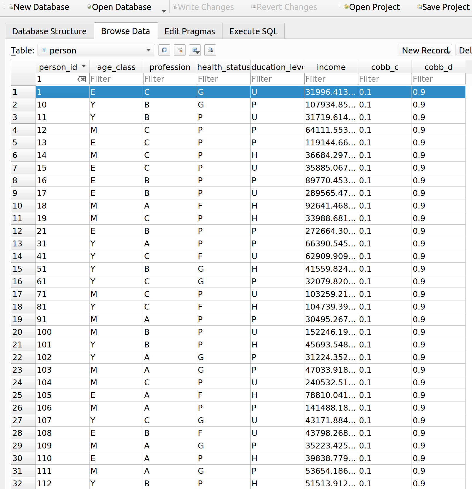
, the same as that derived in Varian. That looks pretty useful. However, Sympy’s documentation is massive, at over 2000 pages. It might take some time to learn it, even if it just involves me grabbing what I need. Since I can make do without calculus for the time being, I’ll save this for another day.

Posted in: Actuarial, Mathematics, MIES

No: 136: MIES – Personal Budget Constraints, Taxes, and Subsidies

2 June, 2020 9:08 PM / 1 Comment / Gene Dan

This entry is part of a series dedicated to MIES – a miniature insurance economic simulator. The source code for the project is available on GitHub.

Current Status

Last week, I demonstrated the first simulation of MIES. Although it can run indefinitely without intervention on my part, I’ve made a lot of assumptions that aren’t particularly realistic – such as the ability of insureds to buy as much insurance as they wanted without any kind of constraint on affordability. I’ll address this today by implementing a budget constraint, a concept typically introduced during the first week of a second year economics course.

Most of the economic theory that I’ll be introducing to MIES for the time being comes from two books: Hal Varian’s Intermediate Microeconomics, a favorite of mine from school, and Zweifel and Eisen’s Insurance Economics, which at least according to the table of contents and what little I’ve read so far, seems to have much of the information I’d want to learn about for MIES.

I’m going to avoid repeating much of what can already be read in these books, so just an fyi, these are the sources I’m drawing from. My goals are to refresh my knowledge of economics as I read and then implement what I see in Python to add features to MIES.

The Economics Module

I’ve added a new module to the project, econtools.py. For now, this will contain the classes for exploring economics concepts with MIES, but seeing how much it has grown in just one week, it’s likely I’ll break it up in the near future. I’ll go over the first classes I’ve written for the module, those written for the budget constraint: Budget, Good, Tax, and Subsidy.

Budget Constraint

Those of you who have taken an economics course ought to find the following graph, a budget constraint, familiar:

As in the real world, there are only two goods that a person can possibly buy:

  1. Insurance
  2. Non-insurance

The budget constraint represents the set of possible allocations between insurance and non-insurance, aka all other goods. This can be represented by an equation as well:

    \[p_1 x_1 + p_2 x_2 = m\]

Where each x represents the quantity of each good and each p represents the prices per unit for each good, and m represents income. People can only buy as much insurance as their incomes can support, hence the need for introducing this constraint into MIES for each person. The budget constraint simply shows that in order to buy one dollar more of insurance, you have to spend one dollar less on anything else that you were going to buy with your income.

The price of insurance is often thought of as a rate per unit of exposure, exposure being some kind of denominator to measure risk, such as miles driven, house-years, actuarial exams taken, or really anything you can think of that correlates with a risk that you’d like to charge money for.

Interestingly, there is nothing in the budget constraint as shown above that would prevent someone from insuring something twice or purchasing some odd products like a ‘lose-1-dollar-get-5-dollars back’ multiplier scheme. I’m not sure if these are legal or simply just discouraged by insurers as I’ve never tried to buy such a product myself or seen it advertised. I could imagine why insurers would not to sell these things – maybe due to the potential for fraud or the fact that an insured thing is 100% correlated with itself. On the other hand, a company might be able to compensate for these risks by simply charging more money to accept them. Regardless, if these products are really undesirable, I’d rather let the simulations demonstrate the impact of unrestricted product design than to have it constrained from the start. I’ll save that for another day.

The budget constraint is modeled with the Budget class in econtools.py. It accepts the goods to be allocated along with other relevant information, such as their prices and the income of the person for whom we are modeling the budget. You’ll see that the class contains references to the other component classes (Good, Tax, Subsidy) which are explained later:

Python
1
2
3
4
5
6
7
8
9
10
11
12
13
14
15
16
17
18
19
20
21
22
23
24
25
26
27
28
29
30
31
32
33
34
35
36
37
38
39
40
41
42
43
44
45
46
47
48
49
50
51
52
53
54
55
56
57
58
59
60
61
62
63
64
65
66
67
68
69
70
71
72
73
74
75
76
77
78
79
80
81
82
83
84
85
86
87
88
89
90
91
92
93
94
95
96
97
98
99
100
101
102
103
104
105
106
107
108
109
110
111
112
113
114
115
116
117
118
119
120
121
122
123
124
125
126
127
128
129
130
131
132
133
134
135
136
137
138
class Budget:
    def __init__(self, good_x, good_y, income, name):
        self.good_x = good_x
        self.good_y = good_y
        self.income = income
        self.x_lim = self.income / (min(self.good_x.adjusted_price, self.good_x.price)) * 1.2
        self.y_lim = self.income / (min(self.good_y.adjusted_price, self.good_y.price)) * 1.2
        self.name = name
 
    def get_line(self):
        data = pd.DataFrame(columns=['x_values', 'y_values'])
        data['x_values'] = np.arange(int(min(self.x_lim, self.good_x.ration)) + 1)
 
        if self.good_x.tax:
            data['y_values'] = self.calculate_budget(
                good_x_price=self.good_x.price,
                good_y_price=self.good_y.price,
                good_x_adj_price=self.good_x.adjusted_price,
                good_y_adj_price=self.good_y.adjusted_price,
                m=self.income,
                modifier=self.good_x.tax,
                x_values=data['x_values']
            )
        elif self.good_x.subsidy:
            data['y_values'] = self.calculate_budget(
                good_x_price=self.good_x.price,
                good_y_price=self.good_y.price,
                good_x_adj_price=self.good_x.adjusted_price,
                good_y_adj_price=self.good_y.adjusted_price,
                m=self.income,
                modifier=self.good_x.subsidy,
                x_values=data['x_values']
            )
        else:
            data['y_values'] = (self.income / self.good_y.adjusted_price) - \
                       (self.good_x.adjusted_price / self.good_y.adjusted_price) * data['x_values']
 
        return {'x': data['x_values'],
                'y': data['y_values'],
                'mode': 'lines',
                'name': self.name}
 
    def calculate_budget(
            self,
            good_x_price,
            good_y_price,
            good_x_adj_price,
            good_y_adj_price,
            m,
            modifier,
            x_values
    ):
        y_int = m / good_y_price
        slope = -good_x_price / good_y_price
        adj_slope = -good_x_adj_price / good_y_adj_price
        base_lower = int(modifier.base[0])
        base_upper = int(min(modifier.base[1], max(m / good_x_price, m / good_x_adj_price)))
        modifier_type = modifier.style
 
        def lump_sum(x):
            if x in range(modifier.amount + 1):
                x2 = y_int
                return x2
            else:
                x2 = y_int + adj_slope * (x - modifier.amount)
                return x2
 
        def no_or_all_adj(x):
            x2 = y_int + adj_slope * x
            return x2
 
        def beg_adj(x):
            if x in range(base_lower, base_upper + 1):
                x2 = y_int + adj_slope * x
                return x2
            else:
                x2 = y_int + slope * (x + (adj_slope/slope - 1) * base_upper)
                return x2
 
        def mid_adj(x):
            if x in range(base_lower):
                x2 = y_int + slope * x
                return x2
            elif x in range(base_lower, base_upper + 1):
                x2 = y_int + adj_slope * (x + (slope/adj_slope - 1) * (base_lower - 1))
                return x2
            else:
                x2 = y_int + slope * (x + (adj_slope/slope - 1) * (base_upper - base_lower + 1))
                return x2
 
        def end_adj(x):
            if x in range(base_lower):
                x2 = y_int + slope * x
                return x2
            else:
                x2 = y_int + adj_slope * (x + (slope/adj_slope - 1) * (base_lower - 1))
                print(x, x2)
                return x2
 
        cases = {
            'lump_sum': lump_sum,
            'no_or_all': no_or_all_adj,
            'beg_adj': beg_adj,
            'mid_adj': mid_adj,
            'end_adj': end_adj,
        }
 
        if modifier_type == 'lump_sum':
            option = 'lump_sum'
        elif modifier.base == [0, np.Inf]:
            option = 'no_or_all'
        elif (modifier.base[0] == 0) and (modifier.base[1] < max(m/good_x_price, m/good_x_adj_price)):
            option = 'beg_adj'
        elif (modifier.base[0] > 0) and (modifier.base[1] < max(m/good_x_price, m/good_x_adj_price)):
            option = 'mid_adj'
        else:
            option = 'end_adj'
 
        adj_func = cases[option]
        print(option)
        return x_values.apply(adj_func)
 
    def show_plot(self):
        fig = go.Figure(data=go.Scatter(self.get_line()))
        fig['layout'].update({
            'title': 'Budget Constraint',
            'title_x': 0.5,
            'xaxis': {
                'range': [0, self.x_lim],
                'title': 'Amount of ' + self.good_x.name
            },
            'yaxis': {
                'range': [0, self.y_lim],
                'title': 'Amount of ' + self.good_y.name
            },
            'showlegend': True
        })
        plot(fig)

Goods

The Good class represents things consumers can buy. We can set the price, as well as apply any taxes and subsidies:

1
2
3
4
5
6
7
8
9
10
11
12
13
14
15
16
17
18
19
20
21
22
23
24
25
26
27
28
29
30
31
32
33
34
35
36
37
38
class Good:
    def __init__(
        self,
        price,
        tax=None,
        subsidy=None,
        ration=None,
        name='Good',
    ):
 
        self.price = price
        self.tax = tax
        self.subsidy = subsidy
        self.adjusted_price = self.apply_tax(self.price)
        self.adjusted_price = self.apply_subsidy(self.adjusted_price)
        if ration is None:
            self.ration = np.Inf
        else:
            self.ration = ration
        self.name = name
 
    def apply_tax(self, price):
        if (self.tax is None) or (self.tax.style == 'lump_sum'):
            return price
        if self.tax.style == 'quantity':
            return price + self.tax.amount
        # else, assume ad valorem
        else:
            return price * (1 + self.tax.amount)
 
    def apply_subsidy(self, price):
        if (self.subsidy is None) or (self.subsidy.style == 'lump_sum'):
            return price
        if self.subsidy.style == 'quantity':
            return price - self.subsidy.value
        # else, assume ad valorem
        else:
            return price * (1 - self.subsidy.amount)

Taxes

Taxes can be added to goods via the Tax class:

Python
1
2
3
4
5
class Tax:
    def __init__(self, amount, style, base=None):
        self.amount = amount
        self.style = style
        self.base = base

The tax class has three attributes, the amount, which specifies the amount of tax to be applied, style, which (for lack of a better word) specifies whether the tax is a quantity, value (or ad valorem) tax, or lump-sum tax. A quantity tax is a fixed amount of tax applied to each unit of a good purchased, a value tax is a tax that is proportional to the price of a good, and a lump-sum tax is a one-time tax paid for participating in the market for that good. Finally, the base attribute specifies over what quantities a tax applies (for example, a tax applied to the first 5 units purchased).

To demonstrate, we’ll add three different types of taxes to our insurance, first by specifying the tax details, and then adding them to the goods, we then specify the relevant budget constraints:

Python
1
2
3
4
5
6
7
8
9
10
11
12
13
14
15
16
17
18
19
20
ad_valorem_tax = ec.Tax(amount=1, style='value', base=[0,np.Inf])
quantity_tax = ec.Tax(amount=4, style='quantity', base=[0, np.Inf])
all_other = ec.Good(price=1, name='All Other Goods')
ad_valorem_first_two = ec.Tax(amount=1, style='value', base=[0, 2])
 
insurance_no_tax = ec.Good(price=1, name='Insurance')
insurance_ad_valorem = ec.Good(price=1, tax=ad_valorem_tax, name='Insurance')
insurance_value = ec.Good(price=1, tax=quantity_tax, name='Insurance')
insurance_first_two = ec.Good(price=1, tax=ad_valorem_first_two, name='Insurance')
 
budget_no_tax = ec.Budget(insurance_no_tax, all_other, income=10, name='No Tax')
budget_ad_valorem = ec.Budget(insurance_ad_valorem, all_other, income=10, name='Ad Valorem Tax')
budget_quantity = ec.Budget(insurance_value, all_other, income=10, name='Value Tax')
budget_first_two = ec.Budget(insurance_first_two, all_other, income=10, name='Ad Valorem Tax - First 2')
 
fig = go.Figure()
fig.add_trace(go.Scatter(budget_no_tax.get_line()))
fig.add_trace(go.Scatter(budget_ad_valorem.get_line()))
fig.add_trace(go.Scatter(budget_quantity.get_line()))
fig.add_trace(go.Scatter(budget_first_two.get_line()))

We can now plot the resulting budget constraints on a single graph:

As expected, the no-tax scenario (blue line) allows the insured to purchase the most insurance, indicated by the x-intercept at 10. Contrast this with the most punitive tax, the value tax shown by the green line with an x-intercept at 2. In this scenario, we increase the price of each unit of insurance form 1 to 5, so that the insured can at most afford 2 units of insurance.

Between these two extremes are the two ad valorem taxes that double the price of insurance. However, the purple line is less punitive as it only taxes the first two units of insurance purchased.

Subsidies

Subsidies behave very similarly to taxes, so much so that I have considered either defining them as a single class or both inheriting from a superclass. Instead of penalizing the consumer, subsidies reward the consumer either by lowering the price of a good or by giving away free units of a good:

Python
1
2
3
4
5
class Subsidy:
    def __init__(self, amount, style, base=None):
        self.amount = amount
        self.style = style
        self.base = base

Just like with taxes, we can specify the subsidy amount, style, and quantities to which it applies. For instance, let’s suppose that as part of a risk-management initiative, the government grants 2 free units of insurance to a consumer in the form of a lump sum subsidy:

The subsidy has allowed the consumer to have at least 2 units of insurance without impacting the maximum amount of all other goods they can buy. We also see that the maximum amount of insurance the consumer can purchase has increased by the same amount, from 10 to 12.

MIES Integration

To integrate these classes and make use of the econtools.py module, I’ve made some changes to the existing MIES modules. In last week’s example, income was irrelevant for each person, and therefore they were unconstrained with respect to the amount of insurance they could purchase. Since a budget constraint is only relevant in the form of some kind of limited spending power, I’ve decided to introduce consumer income into MIES.

Income is now determined by a Pareto distribution, though certainly other distributions are possible and more realistic. In the parameters.py module, I’ve added a value of 30000 as the scale parameter for each person:

Python
1
2
3
4
5
6
7
person_params = {
    'age_class': ['Y', 'M', 'E'],
    'profession': ['A', 'B', 'C'],
    'health_status': ['P', 'F', 'G'],
    'education_level': ['H', 'U', 'P'],
    'income': 30000
}

The person SQLite table has also been updated to accept income as a field:

Python
1
2
3
4
5
6
7
8
9
10
11
12
13
14
15
16
17
18
19
20
21
22
23
24
25
26
27
28
29
30
31
32
33
34
35
36
class Person(Base):
    __tablename__ = 'person'
 
    person_id = Column(
        Integer,
        primary_key=True
    )
    age_class = Column(String)
    profession = Column(String)
    health_status = Column(String)
    education_level = Column(String)
    income = Column(Float)
 
    policy = relationship(
        "Policy",
        back_populates="person"
    )
    event = relationship(
        "Event",
        back_populates="person"
    )
 
    def __repr__(self):
        return "<Person(" \
               "age_class='%s', " \
               "profession='%s', " \
               "health_status='%s', " \
               "education_level='%s'" \
               "income='%s'" \
               ")>" % (
                self.age_class,
                self.profession,
                self.health_status,
                self.education_level,
                self.income
                )

And finally, I’ve added a method to the environment class to assign incomes to each person by drawing from the Pareto distribution using the scale parameter:

Python
1
2
3
4
5
6
7
8
9
10
11
12
13
14
15
16
17
18
19
20
21
22
23
24
25
26
27
28
29
30
31
32
33
    def make_population(self, n_people):
        age_class = pm.draw_ac(n_people)
        profession = pm.draw_prof(n_people)
        health_status = pm.draw_hs(n_people)
        education_level = pm.draw_el(n_people)
        income = pareto.rvs(
            b=1,
            scale=pm.person_params['income'],
            size=n_people,
        )
 
        population = pd.DataFrame(list(
            zip(
                age_class,
                profession,
                health_status,
                education_level,
                income
            )
        ), columns=[
            'age_class',
            'profession',
            'health_status',
            'education_level',
            'income'
        ])
 
        population.to_sql(
            'person',
            self.connection,
            index=False,
            if_exists='append'
        )

This results in a mean income of five figures with some high-earning individuals making a few million dollars per year. To examine the budget constraint for a single person in MIES, we can do so by running two iterations of the simulation and then querying the database:

Python
1
2
3
4
5
6
7
8
9
10
11
12
13
14
15
16
17
18
19
20
21
22
23
24
25
26
27
28
29
30
31
32
33
34
35
36
37
38
39
40
import pandas as pd
import datetime as dt
import sqlalchemy as sa
import econtools as ec
from SQLite.schema import Person, Policy, Base, Company, Event
from sqlalchemy.orm import sessionmaker
from entities import God, Broker, Insurer
import numpy as np
import plotly.graph_objects as go
from plotly.offline import plot
 
 
pd.set_option('display.max_columns', None)
 
 
engine = sa.create_engine('sqlite:///MIES_Lite.db', echo=True)
Session = sessionmaker(bind=engine)
Base.metadata.create_all(engine)
 
gsession = Session()
 
 
ahura = God(gsession, engine)
ahura.make_population(1000)
 
pricing_date = dt.date(1, 12, 31)
 
 
rayon = Broker(gsession, engine)
company_1 = Insurer(gsession, engine, 4000000, Company, 'company_1')
company_1_formula = 'severity ~ age_class + profession + health_status + education_level'
pricing_status = 'initial_pricing'
free_business = rayon.identify_free_business(Person, Policy, pricing_date)
companies = pd.read_sql(gsession.query(Company).statement, engine.connect())
 
rayon.place_business(free_business, companies, pricing_status, pricing_date, company_1)
ahura.smite(Person, Policy, pricing_date + dt.timedelta(days=1))
company_1.price_book(Person, Policy, Event, company_1_formula)
pricing_status = 'renewal_pricing'
rayon.place_business(free_business, companies, pricing_status, pricing_date, company_1)

When we query the person table, we can see that the person we are interested in (id=1) has an income of about 56k per year:

We can also see that their premium upon renewal was about 21k, almost half their income and much higher than the original premium of 4k:

Let’s look at the events table to see why their premium is so high. It looks like they had a loss of about 174k, so the insurance up to this point has at least been worth their while:

We can now query the relevant information about this person, and use econtools.py to graph their budget constraint prior to and during renewal:

Python
1
2
3
4
5
6
7
8
9
10
11
12
13
14
15
16
17
18
19
20
21
22
23
24
25
26
27
28
29
30
31
32
33
34
35
36
37
38
39
40
41
42
43
44
45
46
47
48
49
myquery = gsession.query(Person.person_id, Person.income, Policy.policy_id, Policy.premium).\
    outerjoin(Policy, Person.person_id == Policy.person_id).\
    filter(Person.person_id == str(1)).\
    filter(Policy.policy_id == str(1001))
 
my_person = pd.read_sql(myquery.statement, engine.connect())
 
my_person
 
all_other = ec.Good(price=1, name="All Other Goods")
price = my_person['premium'].loc[0]
id = my_person['person_id'].loc[0]
income = my_person['income'].loc[0]
renewal = ec.Good(price=price, name="Insurance")
 
original = ec.Good(price=4000, name="Insurance")
budget_original = ec.Budget(good_x=original, good_y=all_other, income=income, name='Orginal Budget')
renewal_budget = ec.Budget(good_x=renewal, good_y=all_other, income=income, name='Renewal Budget')
 
fig = go.Figure()
fig.add_trace(go.Scatter(budget_original.get_line()))
fig.add_trace(go.Scatter(renewal_budget.get_line()))


fig['layout'].update({
            'title': 'Budget Constraint',
            'title_x': 0.5,
            'xaxis': {
                'range': [0, 20],
                'title': 'Amount of Insurance'
            },
            'yaxis': {
                'range': [0, 60000],
                'title': 'Amount of All Other Goods'
            },
            'showlegend': True,
            'legend': {
                'x': .71,
                'y': 1
            },
            'width': 590,
            'height': 450,
            'margin': {
                'l':10
            }
        })
 
fig.write_html('mies_budget.html', auto_open=True)

This insured used to be able to afford about 14 units of insurance prior to their large claim. Upon renewal, their premium went up drastically which led to a big drop in affordability, as indicated by the red line. Now they can only afford a little more than 2 units of insurance.

Further Improvements

The concept of utility builds upon the budget constraint by answering the question – given a budget, what is the optimal allocation of goods one can purchase? I think this will be a bit harder and may take some time to program. As I’ve worked on this, I’ve found my programming stints to fall into three broad categories:

  1. Economic Theory
  2. Insurance Operations
  3. Refactoring

Every now and then after adding stuff to MIES, the code will get messy and the object dependencies more complex than they need to be, therefore, I ought to spend a week here or there just cleaning up the code. Sometimes I’ll stop to work on some practice problems to strengthen my theoretical knowledge, which I suspect I’ll need to do soon since I need a refresher on partial derivatives, which are used to find optimal consumption bundles.

Posted in: Actuarial, Mathematics, MIES

Archives

  • September 2023
  • February 2023
  • January 2023
  • October 2022
  • March 2022
  • February 2022
  • December 2021
  • July 2020
  • June 2020
  • May 2020
  • May 2019
  • April 2019
  • November 2018
  • September 2018
  • August 2018
  • December 2017
  • July 2017
  • March 2017
  • November 2016
  • December 2014
  • November 2014
  • October 2014
  • August 2014
  • July 2014
  • June 2014
  • February 2014
  • December 2013
  • October 2013
  • August 2013
  • July 2013
  • June 2013
  • March 2013
  • January 2013
  • November 2012
  • October 2012
  • September 2012
  • August 2012
  • July 2012
  • June 2012
  • May 2012
  • April 2012
  • March 2012
  • February 2012
  • January 2012
  • December 2011
  • September 2011
  • August 2011
  • July 2011
  • June 2011
  • January 2011
  • December 2010
  • October 2010
  • September 2010
  • August 2010
  • June 2010
  • May 2010
  • April 2010
  • March 2010
  • September 2009
  • August 2009
  • May 2009
  • December 2008

Categories

  • Actuarial
  • Cycling
  • Logs
  • Mathematics
  • MIES
  • Music
  • Uncategorized

Links

Cyclingnews
Jason Lee
Knitted Together
Megan Turley
Shama Cycles
Shama Cycles Blog
South Central Collegiate Cycling Conference
Texas Bicycle Racing Association
Texbiker.net
Tiffany Chan
USA Cycling
VeloNews

Texas Cycling

Cameron Lindsay
Jacob Dodson
Ken Day
Texas Cycling
Texas Cycling Blog
Whitney Schultz
© Copyright 2025 - Gene Dan's Blog
Infinity Theme by DesignCoral / WordPress