The release of FASLR v0.0.8 incorporates a second loss reserving technique into the application – the expected loss technique. This technique is commonly used to estimate ultimate losses for new lines of business or those for which we do not have much data. It’s been a long time since my last update, but I’m excited to continue a project that, besides being used to pad my resume, has brought me into contact with some interesting and innovative members of our profession.
For those wondering what I’ve been up to last year, I spent a good chunk of it writing my first paper for the CAS – Practitioners’ Guide to Building Actuarial Reserving Workflows Using Chainladder-Python, co-authored with John Bogaardt and Kenneth Hsu.
If you are new to FASLR, it stands for Free Actuarial System for Loss Reserving. If you are more interested in discovering FASLR’s capabilities, you can browse previous posts about the project on this blog. You are also free to browse the source code on the CAS GitHub or view the documentation on the project’s website.
Background
By itself, the expected claims technique is simple – it involves an apriori expectation (aka guess) on what ultimate losses will be, and then derives the IBNR estimate by subtracting the incurred losses to date. In its purest form, it can simply be a straight up guess as to what the ultimate losses are, but from a practical standpoint (and to make actuarial exams more challenging) there are some variations on the technique that make use of the observed claims to have some grounding in reality.
To include this technique as a new feature in FASLR, I adapted Friedland’s example that applies the techinque to an Auto BI line of business at an insurer named XYZ. I chose this example because it has several characteristics that make it well-suited for testing in a real-world environment:
- A mixed selection of loss ratios using a blend of loss ratio averaging techniques.
- The use of premium and loss trends, a feature which can also be applied to other techniques.
- Incomplete values in the loss triangles.
- The application of the technique over all accident years, as opposed to just a single year (as seen in other examples in the text).
The most challenging part of this exercise was reproducing Friedland’s application of premium and loss indexes, which, from the paper, was difficult to interpret since it involves 2-dimensional indexes, bringing each accident year to the level of every other accident year.
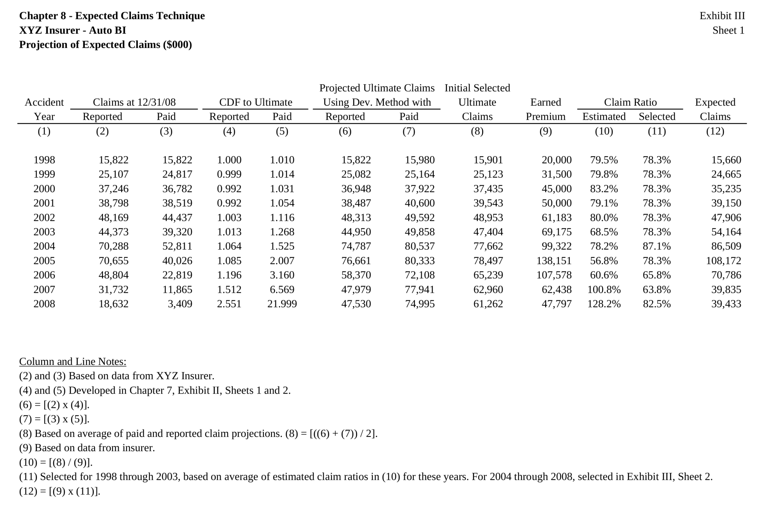
Below, is the exhibit that we seek to reproduce, which shows the selection of initial and final ultimate losses, with some modifications to enhance the user experience. Note that my numbers will differ slightly from hers due to differing rounding practices between her paper and my application.
Trending
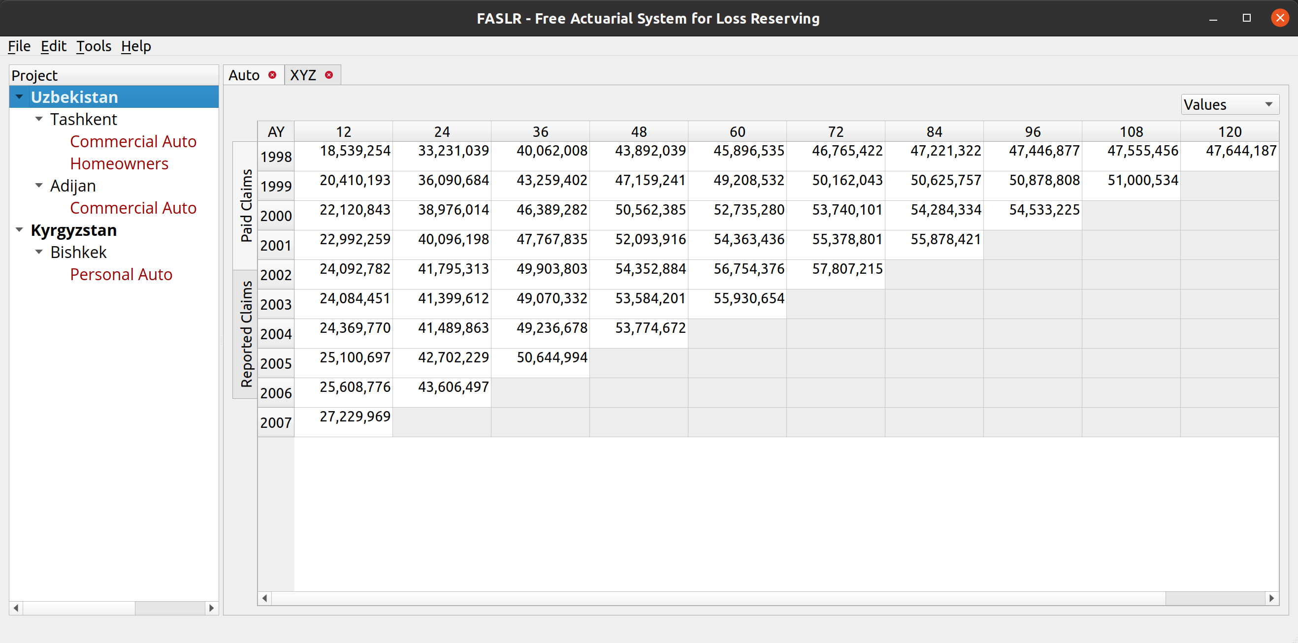
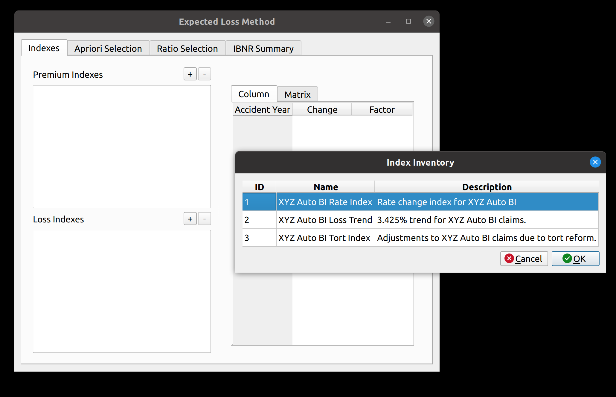
FASLR v0.0.8 adds a loss and premium trending widget. The widget has 2 main subsections. The subsection to the left of the splitter contains two list views that allow us to add premium and loss indexes, respectively. The subsection to the right of the splitter allows one to preview the index(es) that they have added. The plus/minus buttons open up a dialog from which we can insert indexes to the model. This list shown within the dialog box is obtained by querying a database that contains all the indexes uploaded to the application.
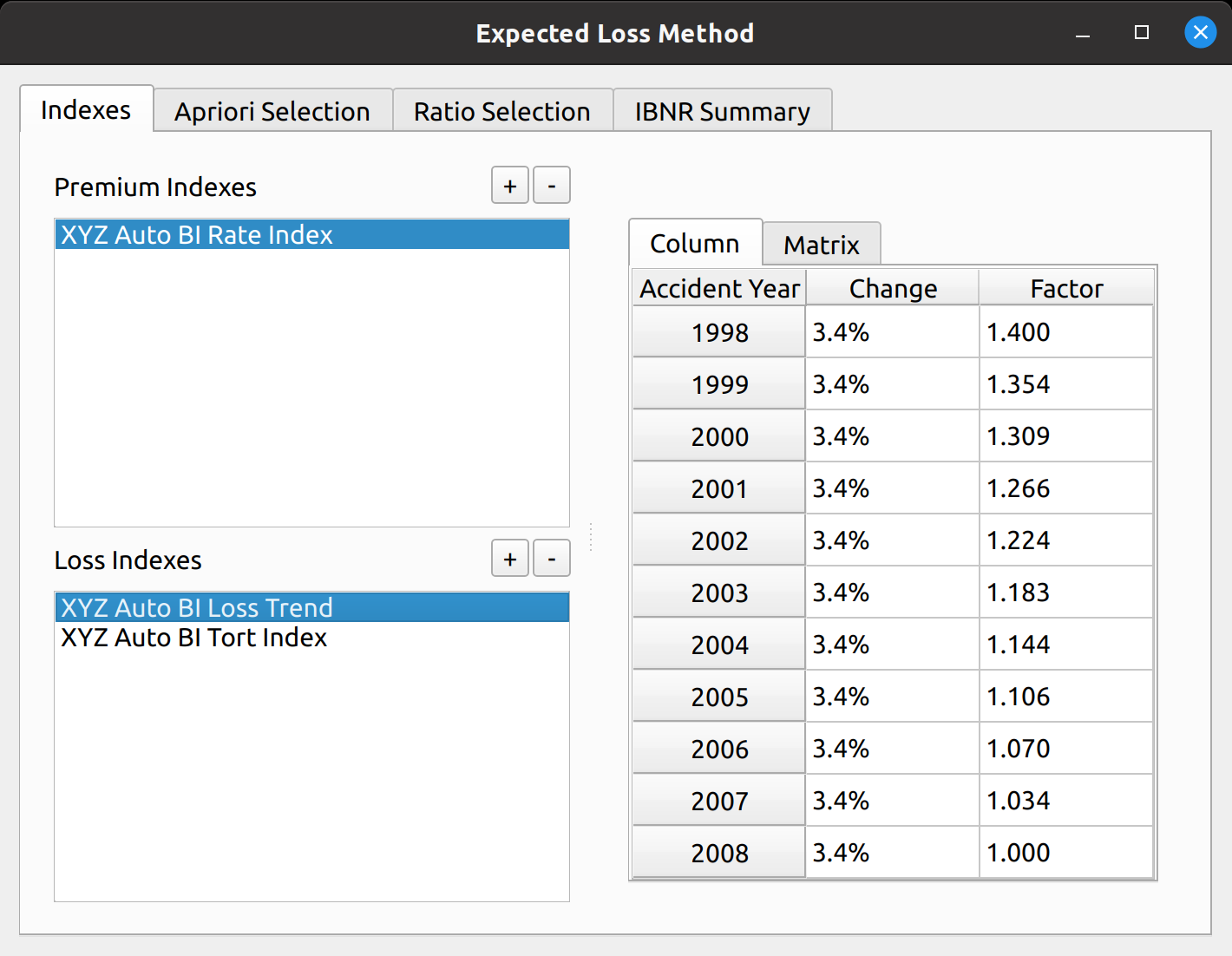
For our example, we add one premium trend index, and two loss indexes: a 3.425% Auto BI loss trend and an index to adjust losses for tort reform. Once this is done, the preview section gets populated. The preview section has two tabs to visualize the adjustment factors. The “Column” tab shows the factors to bring each accident year to the level of the latest accident year.
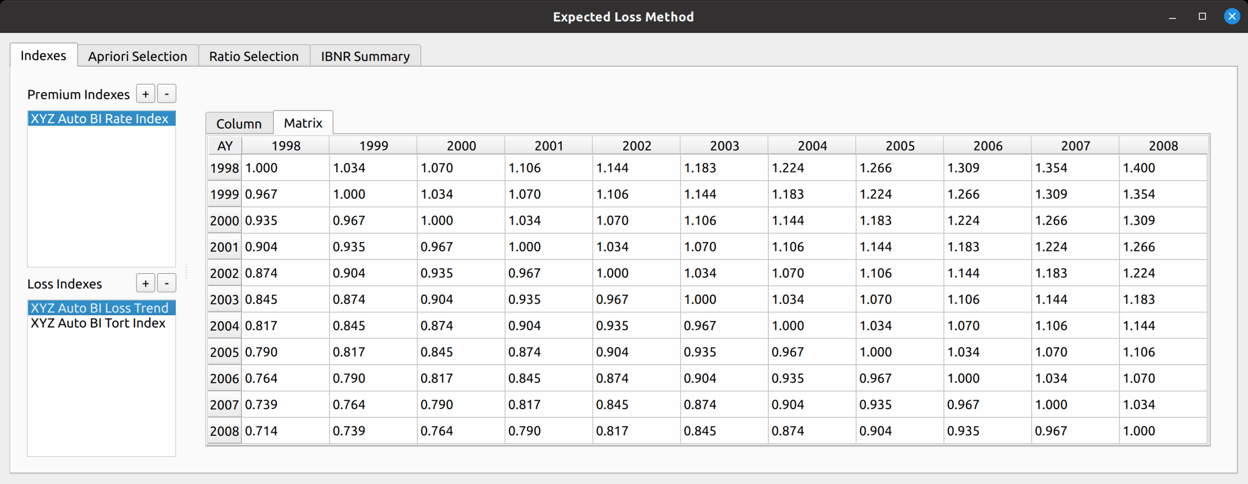
The “Matrix” tab shows the index in matrix form, showing a 2-dimension array of factors to bring each accident year to the level of every other accident year as required for Friedland’s example.
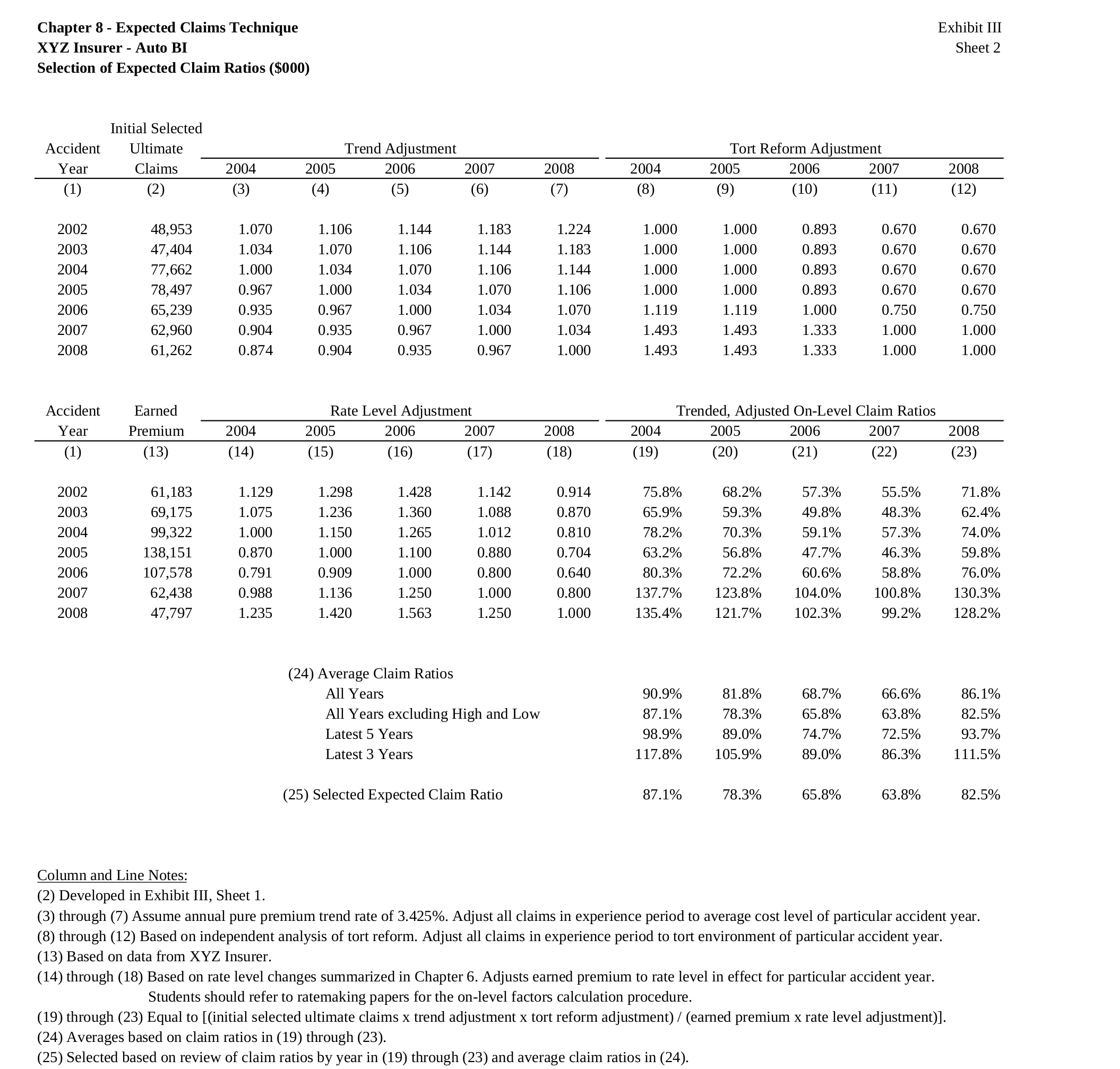
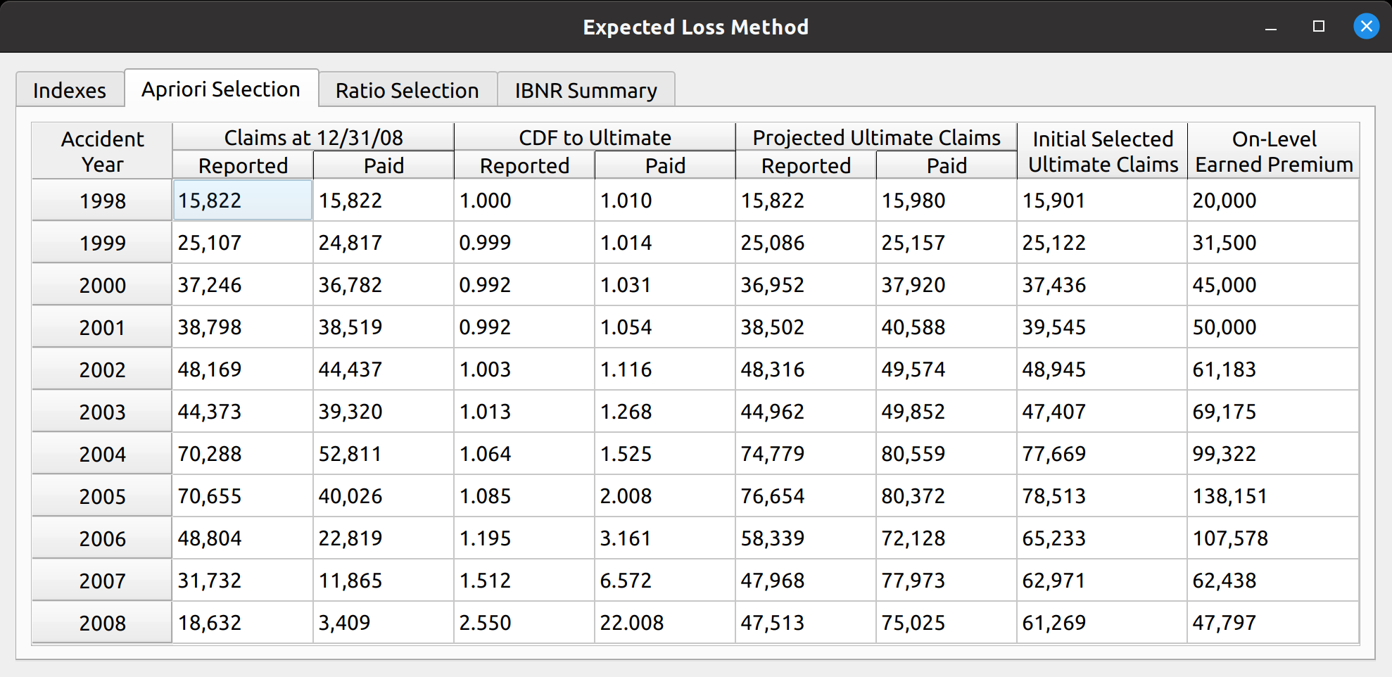
This variation of the expected loss method involves first selecting an initial set of ultimate claims, a straight average of the ultimate losses generated by the chain ladder method applied to paid and reported losses. I have made my own stylistic departure from Friedland’s example by moving the next step – the selection of loss ratios, to the subsequent tab of the model widget.
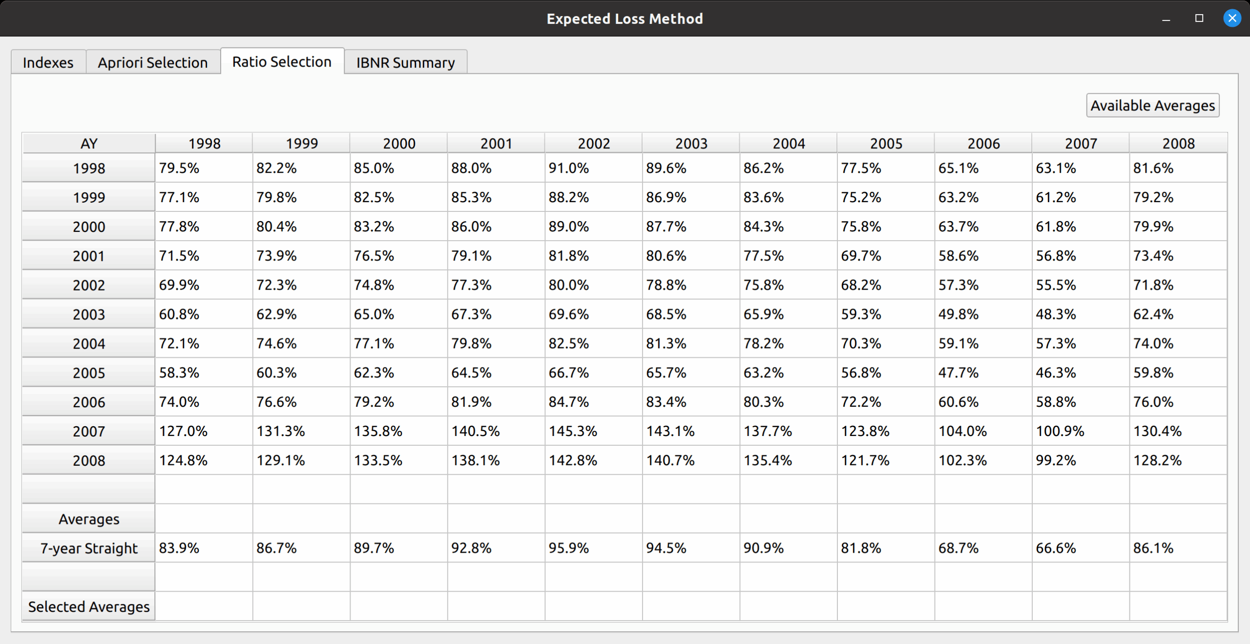
In the next section, the “Ratio Selection Tab”, the trends that we added to the model are applied to the premiums and initial ultimate losses to produce a matrix of loss ratios.
Just like with the chain ladder method, we then produce various averages to help us select our set of apriori loss ratios. The default is the 7-year straight average. Note that this differs from Friedland’s exhibit as my version incorporates more accident years.
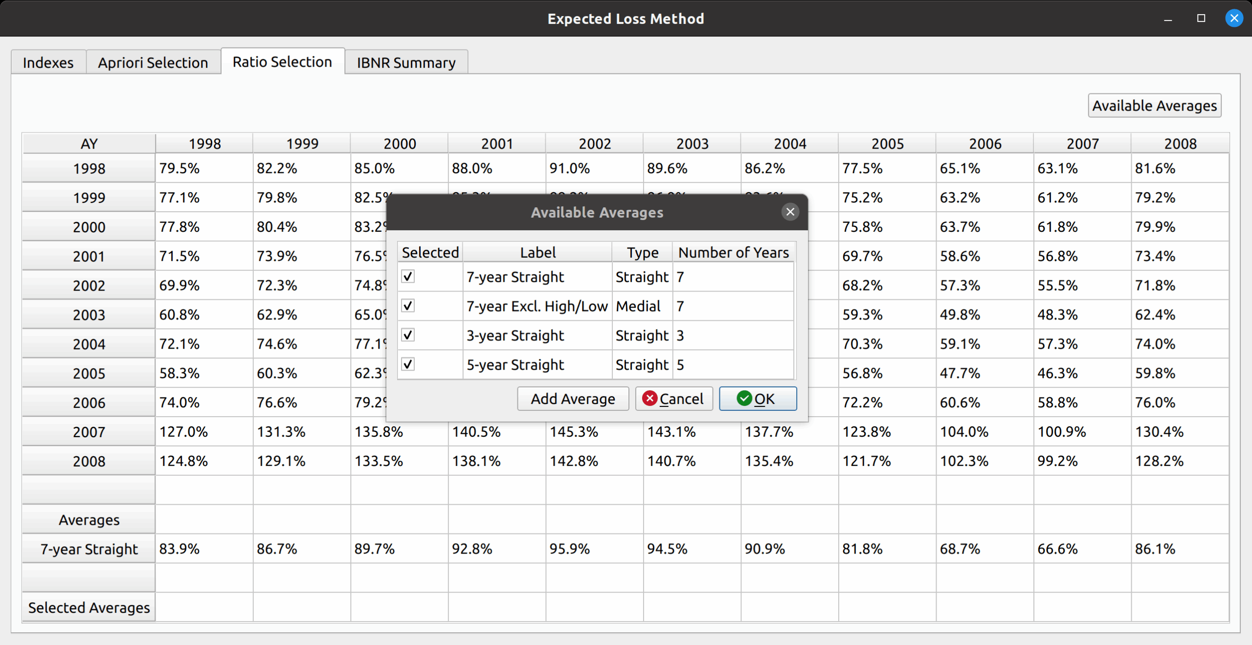
To reproduce Friedland’s exhibit, we can add additional averages by pressing the “Add Averages” button in the upper-right hand corner. This opens a dialog box that lets us add the 7-year medial, 5-year straight, and 3-year straight. In addition to those shown in the table, the model allows us to create new average types (such as a 4-year average, if one desires).
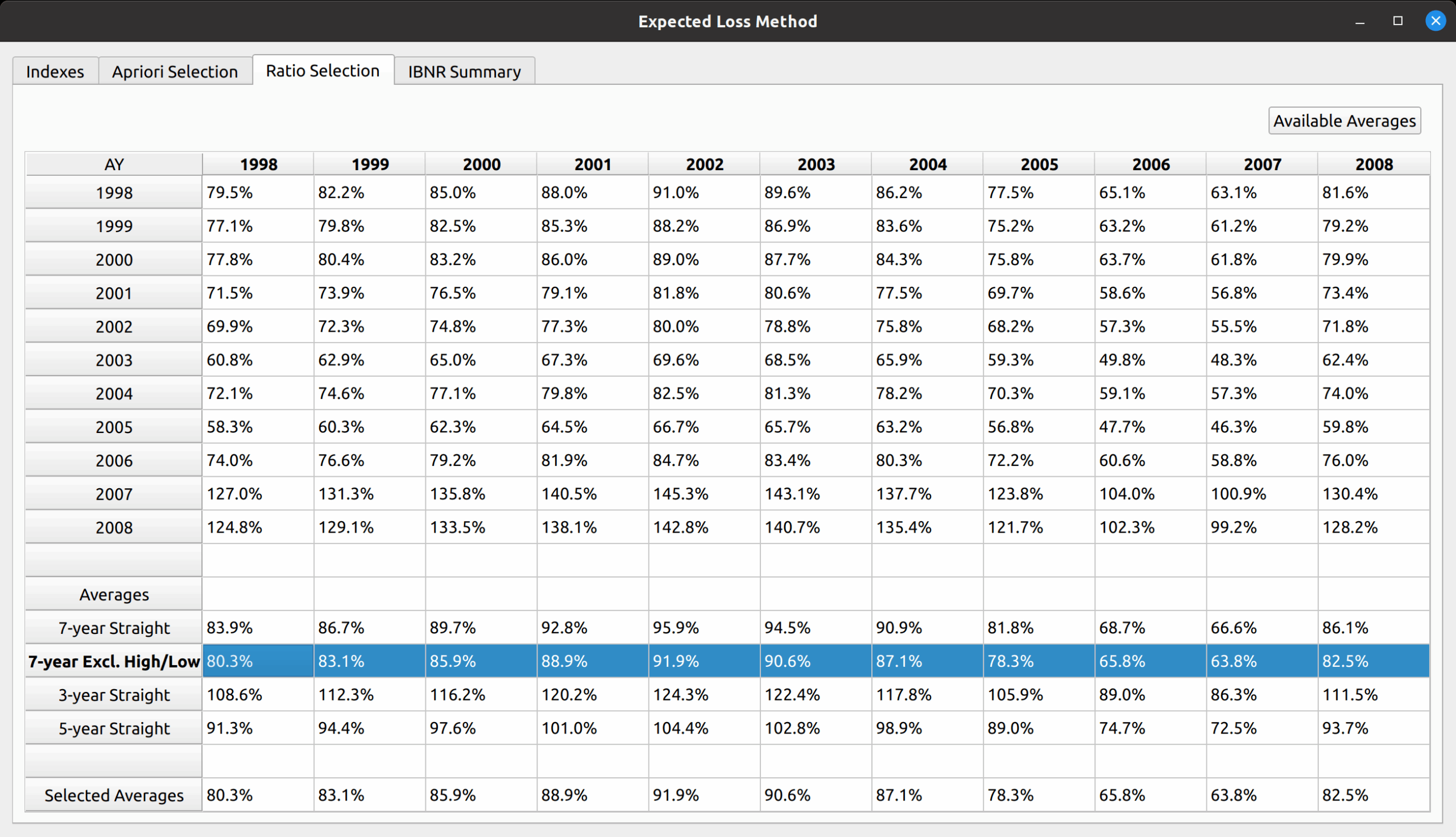
Just like the paper, we first select the 7-year medial average, which copies those averages to the “Selected Averages” row.
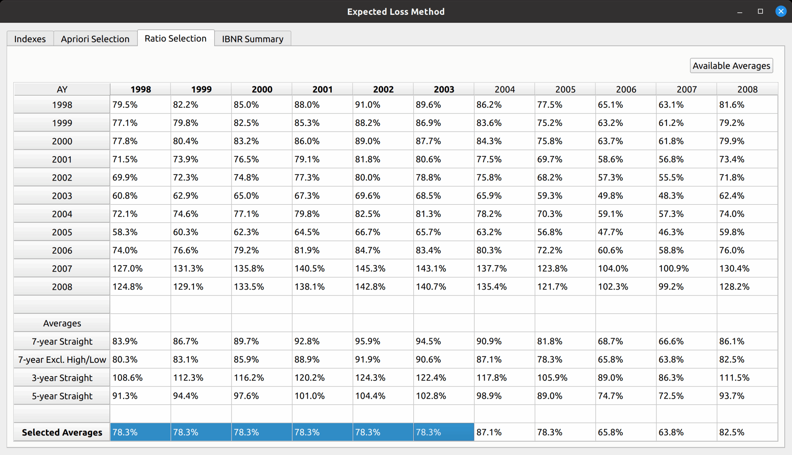
We then complete the reproduction of Friedland’s results by manually inputting the 1998-2003 volume-weighted loss ratio for those years. This can be done simply by copying 78.3% to the corresponding cells.
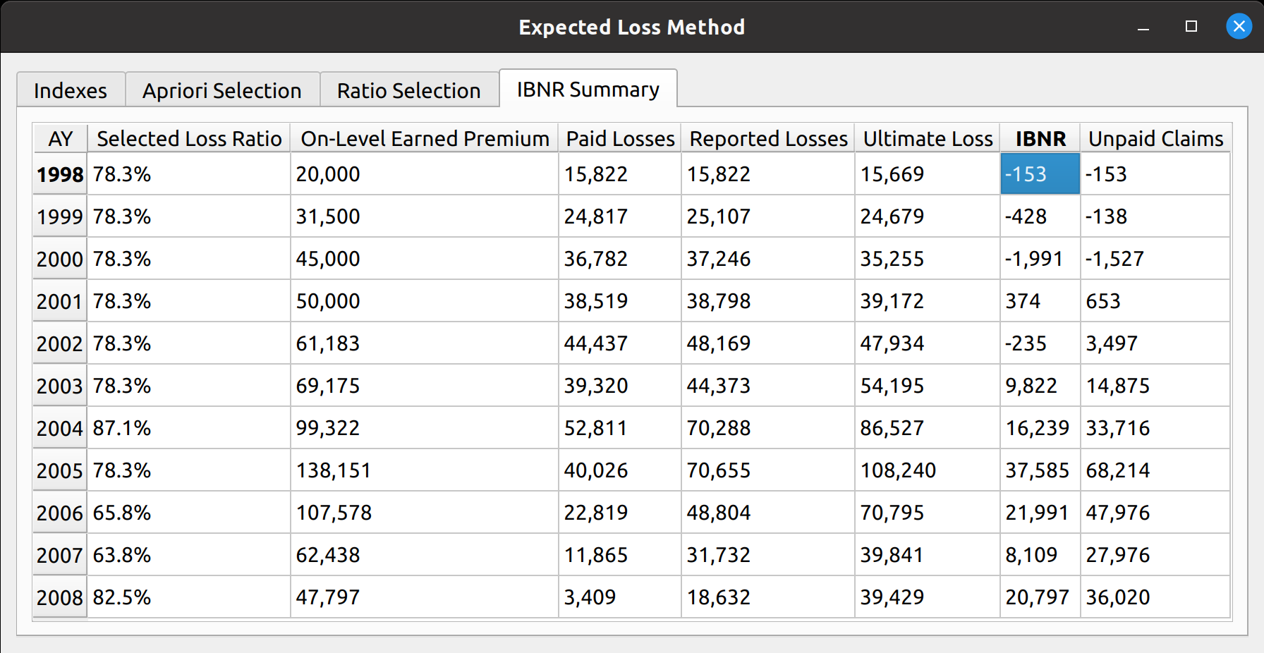
IBNR Summary
The last exhibit, accessed via the IBNR Summary tab, calculates the IBNR by subtracting incurred losses from ultimate losses, and produces an unpaid claim estimate by subtracting paid losses from ultimate losses.