As far as readings go, there wasn’t much to include from the text in today’s post since I just went through a section that covered some basic proof techniques (induction, contradiction, etc.). Tomorrow will be somewhat similar since that section covers general data gathering and manipulation. So today I’ll go over some data I stumbled upon while looking for other texts on graph theory.
The Observatory of Economic Complexity
MIT has some neat data sets here – these contain aggregate trading data for various commodities dating back to 1962. I was interested in looking at crude petroleum movements between countries in the most recent year available, 2014.
Creating a gexf file
Here’s the script I used to generate the gexf file that I imported into gephi. This is pretty much self-contained, and ought to run on your computer as is as long as you have the sqldf package installed. One improvement over previous code is that it fetches the datasets automatically, rather than having me point it out somewhere in my post. I also discovered a useful function called basename() which extracts the file name part of a url string containing a filename.
|
1 2 3 4 5 6 7 8 9 10 11 12 13 14 15 16 17 18 19 20 21 22 23 24 25 26 27 28 29 30 31 32 33 34 35 36 37 38 39 40 41 42 43 44 45 46 47 48 49 50 51 52 53 54 55 56 57 58 59 60 61 62 63 64 65 66 67 68 69 70 71 |
library(sqldf) #source urls for datafiles trade_url <- "http://atlas.media.mit.edu/static/db/raw/year_origin_destination_hs07_6.tsv.bz2" countries_url <- "http://atlas.media.mit.edu/static/db/raw/country_names.tsv.bz2" #extract filenames from urls trade_filename <- basename(trade_url) countries_filename <- basename(countries_url) #download data download.file(trade_url,destfile=trade_filename) download.file(countries_url,destfile=countries_filename) #import data into R trade <- read.table(file = trade_filename, sep = '\t', header = TRUE) country_names <- read.table(file = countries_filename, sep = '\t', header = TRUE) #extract petroleum trade activity from 2014 petro_data <- trade[trade$year==2014 & trade$hs07==270900,] #we want just the exports to avoid double counting petr_exp <- petro_data[petro_data$export_val != "NULL",] #xxb doesn't seem to be a country, remove it petr_exp <- petr_exp[petr_exp$origin != "xxb" & petr_exp$dest != "xxb",] #convert export value to numeric petr_exp$export_val <- as.numeric(petr_exp$export_val) #take the log of the export value to use as edge weight petr_exp$export_log <- log(petr_exp$export_val) petr_exp$origin <- as.character(petr_exp$origin) petr_exp$dest <- as.character(petr_exp$dest) #build edges petr_exp$edgenum <- 1:nrow(petr_exp) petr_exp$edges <- paste('<edge id="', as.character(petr_exp$edgenum),'" source="', petr_exp$origin, '" target="',petr_exp$dest, '" weight="',petr_exp$export_log,'"/>',sep="") #build nodes nodes <- data.frame(id=sort(unique(c(petr_exp$origin,petr_exp$dest)))) nodes <- sqldf("SELECT n.id, c.name FROM nodes n LEFT JOIN country_names c ON n.id = c.id_3char") nodes$nodestr <- paste('<node id="', as.character(nodes$id), '" label="',nodes$name, '"/>',sep="") #build metadata gexfstr <- '<?xml version="1.0" encoding="UTF-8"?> <gexf xmlns:viz="http:///www.gexf.net/1.1draft/viz" version="1.1" xmlns="http://www.gexf.net/1.1draft"> <meta lastmodifieddate="2010-03-03+23:44"> <creator>Gephi 0.7</creator> </meta> <graph defaultedgetype="undirected" idtype="string" type="static">' #append nodes gexfstr <- paste(gexfstr,'\n','<nodes count="',as.character(nrow(nodes)),'">\n',sep="") fileConn<-file("exports_log_norev.gexf") for(i in 1:nrow(nodes)){ gexfstr <- paste(gexfstr,nodes$nodestr[i],"\n",sep="")} gexfstr <- paste(gexfstr,'</nodes>\n','<edges count="',as.character(nrow(petr_exp)),'">\n',sep="") #append edges and print to file for(i in 1:nrow(petr_exp)){ gexfstr <- paste(gexfstr,petr_exp$edges[i],"\n",sep="")} gexfstr <- paste(gexfstr,'</edges>\n</graph>\n</gexf>',sep="") writeLines(gexfstr, fileConn) close(fileConn) |
Generating the graph
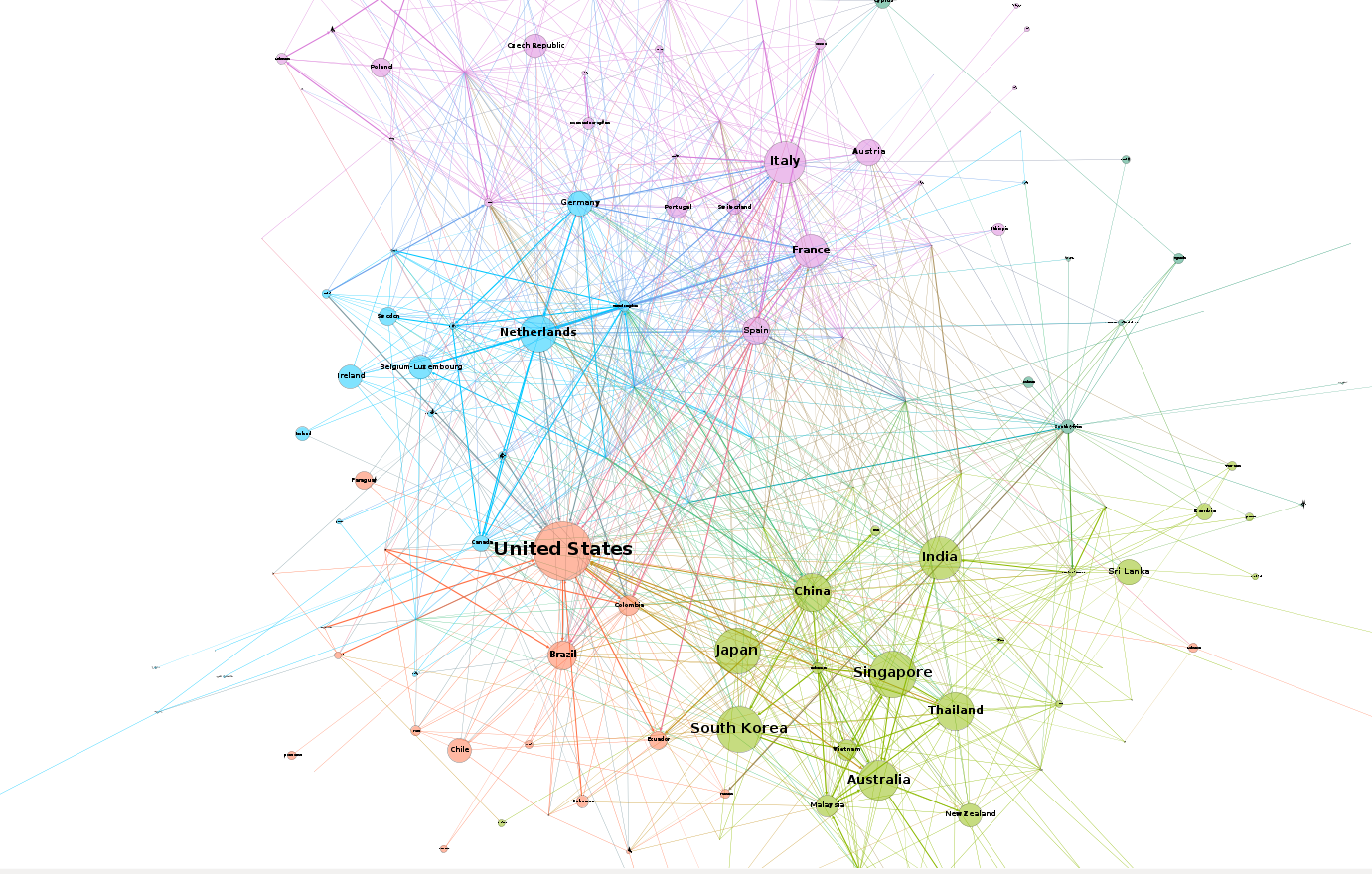
After importing the gexf file, adjusting the graph for eigenvector centrality, and applying some community detection, gephi produced the following result:
Try clicking on the graph – you can zoom in quite a bit to see the countries and edges in detail. I’ve set the graph so that edge width is proportional to the log of the export value, so the higher the trading volume between two countries, the thicker the edge. We can also see that communities are highlighted in the same color – we would intuitively associate these with trading blocs, or groups of countries that work closely together.
In this graph, the node size is proportional to eigenvector centrality. In other words, the larger the node, the more important the country is to the network. To me, this was kind of puzzling. At least in my mind, I would have thought that major exporting nations like Saudi Arabia would have appeared much larger on the graph. However, you can see from the image that countries associated with importing oil dominate the graph.
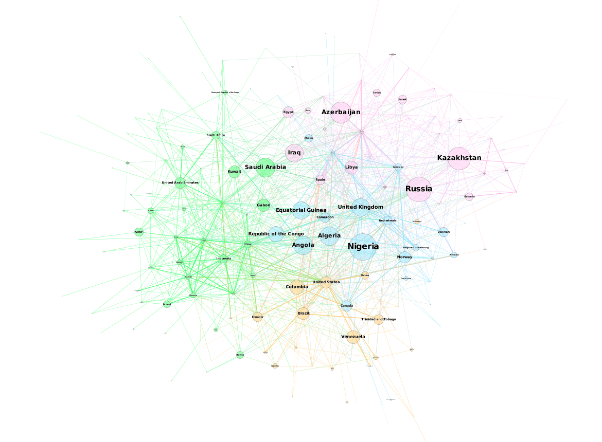
I thought maybe it had to do with the direction of the edges. What we have here is a directed graph – if you look carefully you can see that the edges are actually arrows that point from the exporting country to the importing country. If we reverse the direction of these arrows – that is, recreate the graph from the perspective of money flowing into exporting countries rather than goods flowing out of those countries, we get the following graph:
This graph is a little more consistent with my intuition – we can see that major exporting nations like Saudi Arabia, Iraq, and Azerbaijan appear much larger, while importing nations appear smaller. However, I have to caution myself that just because the graph is consistent with my belief, doesn’t mean I’m right. I’ll have to see if I can further understand centrality as I continue in the course.


would be neat to see an animation of the network over time