• Home
  • Readings
  • Github
  • MIES
  • TmVal
  • About
Gene Dan's Blog

Category Archives: Actuarial

No. 149: FASLR – Import Wizard

23 October, 2022 7:06 PM / Leave a Comment / Gene Dan

The release of FASLR v.0.0.3 brings about two significant changes:

  1. Adding a data import wizard
  2. Upgrading from PyQt5 to PyQt6

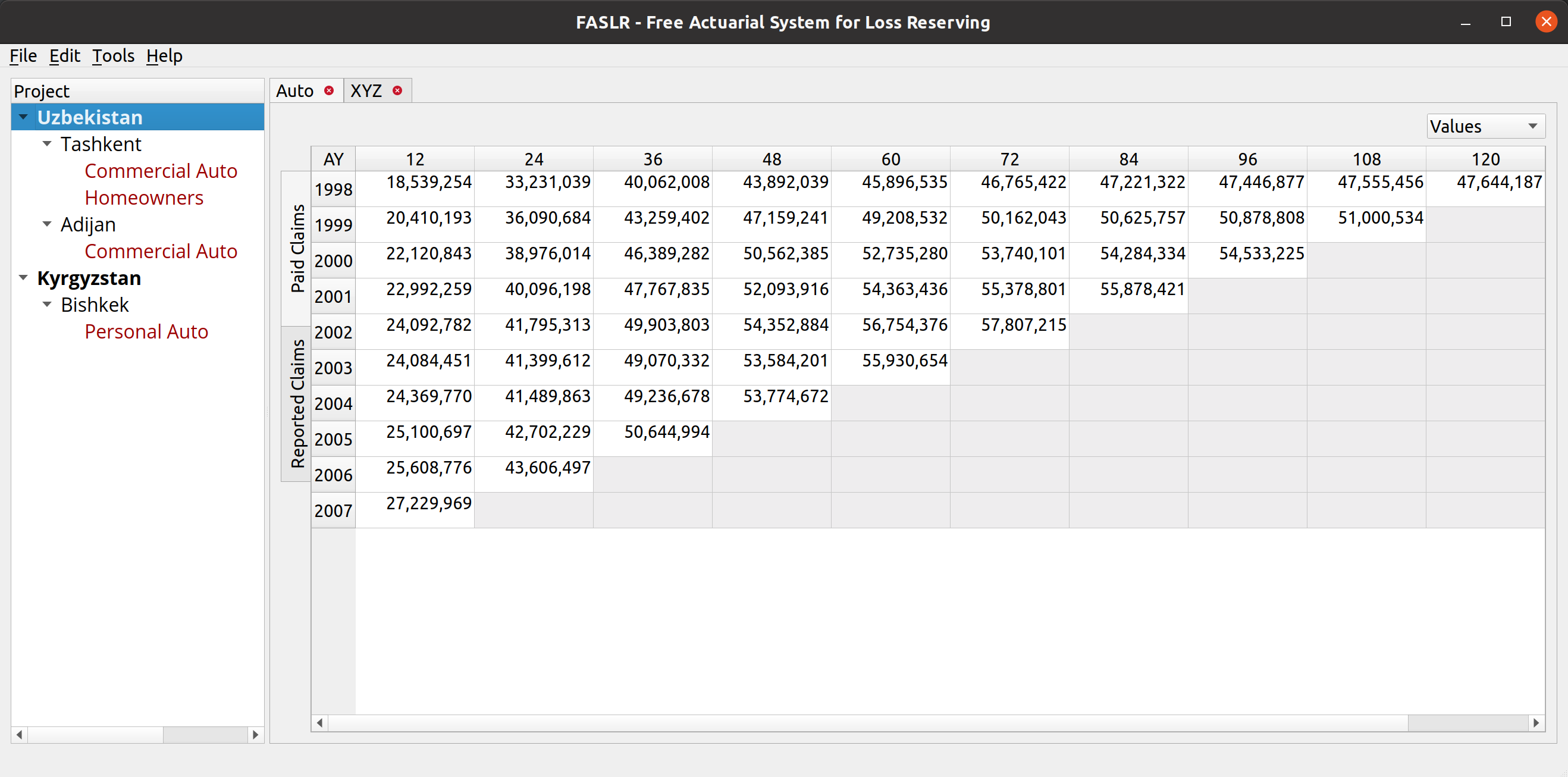
For those new to FASLR, it stands for Free Actuarial System for Loss Reserving, a graphical user interface for the Python chainladder package, both of which are hosted on the Casualty Actuarial Society’s GitHub page. Working on the import wizard has so far, been one of the most enjoyable parts of developing FASLR, not only because I had never imagined myself ever making something like this in my programming journey, but also because my increasing command over the PyQt6 system has allowed me to put the ideas I have visualized in my head onto the computer screen.

Importing Data

Until now, there hasn’t been a way to load external data into FASLR, besides altering the source code to make that happen. Most of what you see in my previous posts on FASLR are examples that can be found in the repo’s demos folder, and illustrate some of program’s existing features on dummy data from actuarial papers. Actually, there still isn’t a way for the user to get data into FASLR, as this post is about the Import Wizard, and not about what happens to the data after you press the ‘OK’ button – that will have to wait for another time.

Anyway, the lack of any kind of import functionality prompted me to begin working on it. Ideally, in-house reserving systems ought to be connected to the company’s loss database, and data should be automatically fed into the system at regular intervals (monthly, quarterly, etc.), negating the need for a manual import wizard to get data into the program. That’s rarely the case however, and even departments that are pretty good at automating that kind of thing will still have the need for their employees to manually insert data in the situations where such automation falls short – such as copying and pasting numbers from Excel or uploading external CSV files. Thus, I decided some kind of import wizard was necessary.

Basic Layout

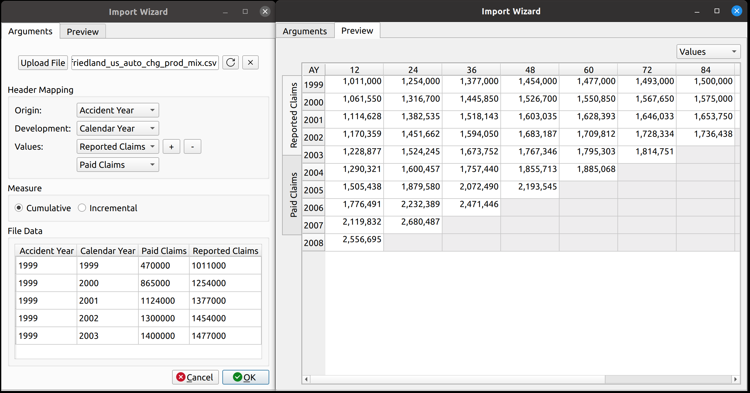
The import wizard has two tabs – one for mapping the external data to its internal FASLR representation, and another to preview the resulting triangle prior to upload. These are labeled “Arguments” and “Preview”, respectively.

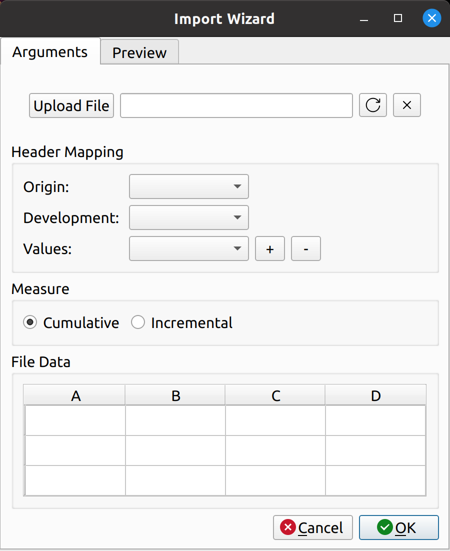
The arguments tab has four main sections:

  • File Upload
  • Header Mapping
  • Measure
  • File Data

The file upload section lets you select a CSV file for import. It has an upload button to the left, a text box in the middle to hold the file path, and two buttons to the right to cancel and refresh the form.

The header mapping section is what allows the user to map the CSV fields, say, “Paid Losses” and “Accident Year” to the triangle fields used by FASLR.

The measure section just indicates whether the triangle should be cumulative or incremental. Most triangles encountered by actuaries are cumulative, so I’ve made that the default. I agonized over what to call this section, since I don’t think there’s a commonly accepted word that actuaries use to describe whether a triangle is cumulative or incremental. “Cumulativeness” or “incrementalness” just sounds weird, so I called the section “measure”, which is subject to change if I or someone else finds something better.

The file data section lets the user view the data in the CSV file, to assist them with mapping the fields.

Uploading Files

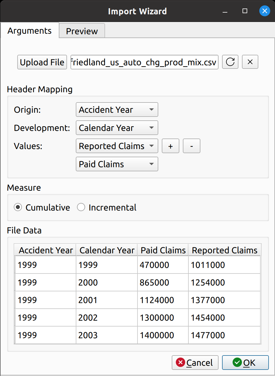
Uploading files is as simple as it gets. You click the upload button, and then the wizard reads in the data and displays it in the File Data section on the bottom. The file headers are read and are then provided as options to map to the triangle fields.

Smart Mapping

The next step is to map the CSV headers to the triangle fields. In chainladder, this is done by providing arguments to the data, origin, development, columns, and cumulative parameters to the Triangle class:

Python
1
2
3
4
5
6
7
8
raa = cl.Triangle(
    raa_df,
    origin="origin",
    development="development",
    columns="values",
    cumulative=True,
)
raa

Notice how the dropdown fields correspond to these arguments. This is how FASLR generates the triangles behind the scenes. It would be tedious, however, to map the CSV headers to these arguments manually every time, so the import wizard provides a smart mapping to automatically pick certain commonly used columns. For example, accident year often corresponds to “origin” and something like paid losses would often correspond to “values”. There is no special AI here, this is just done via business rules using pre-populated dictionaries that can be configured and customized by the user.

The user can also select the number of value columns to be used for the triangle by clicking the “+” and “-” buttons – for example, if the data file has both paid and reported losses, you can increase the number of columns to account for this.
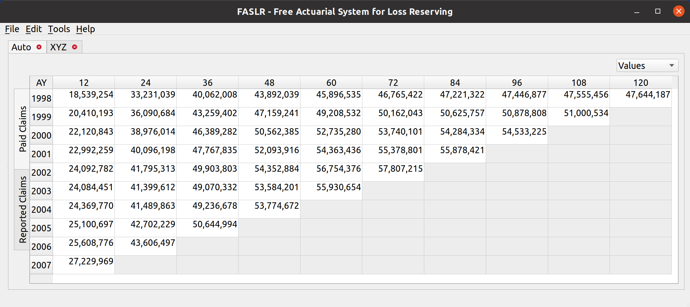
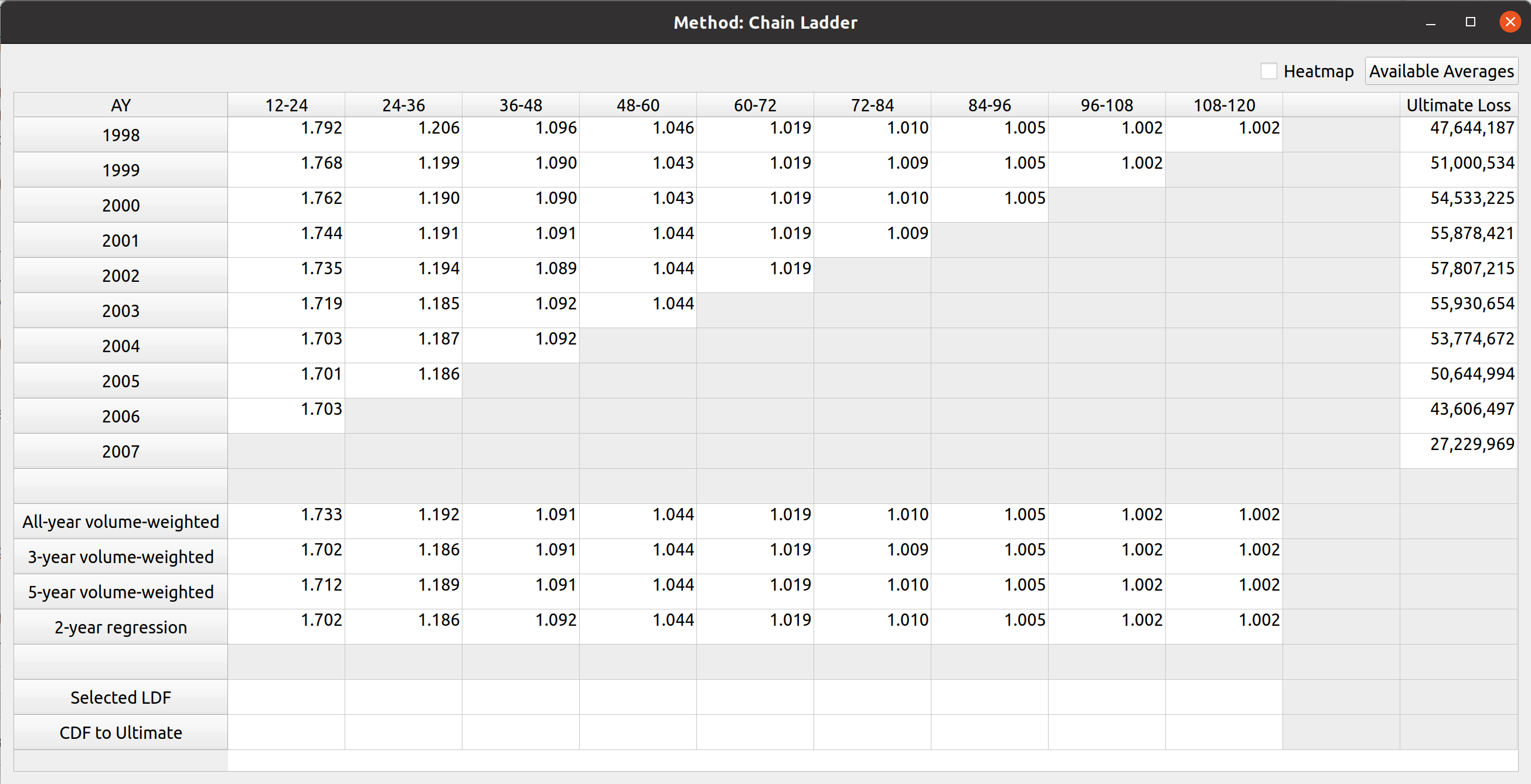
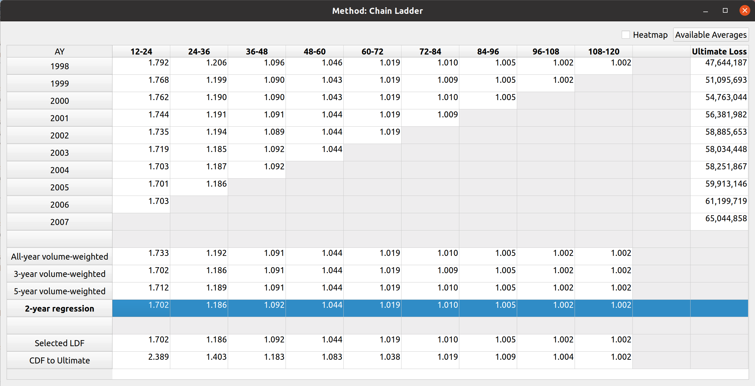
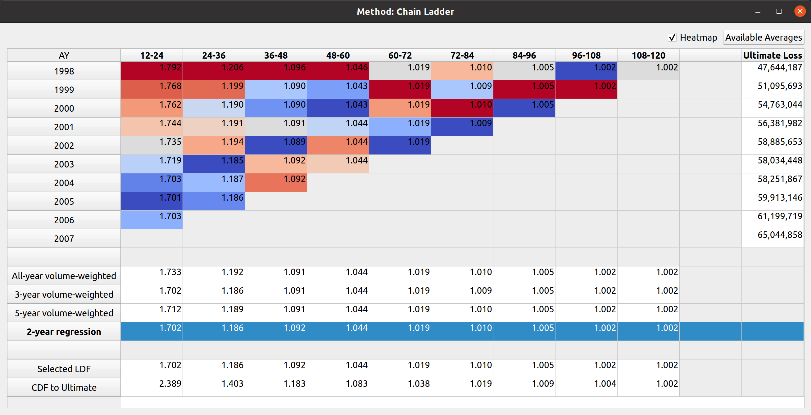
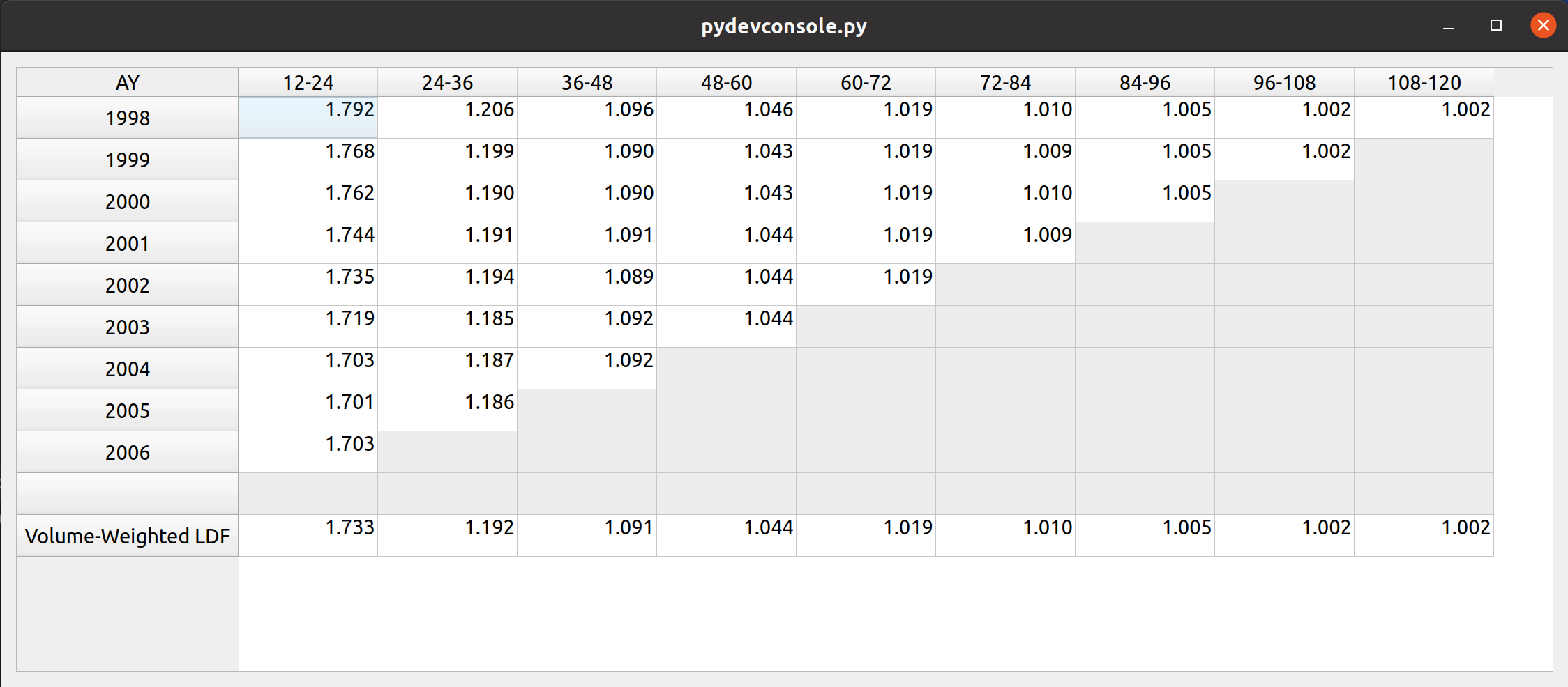
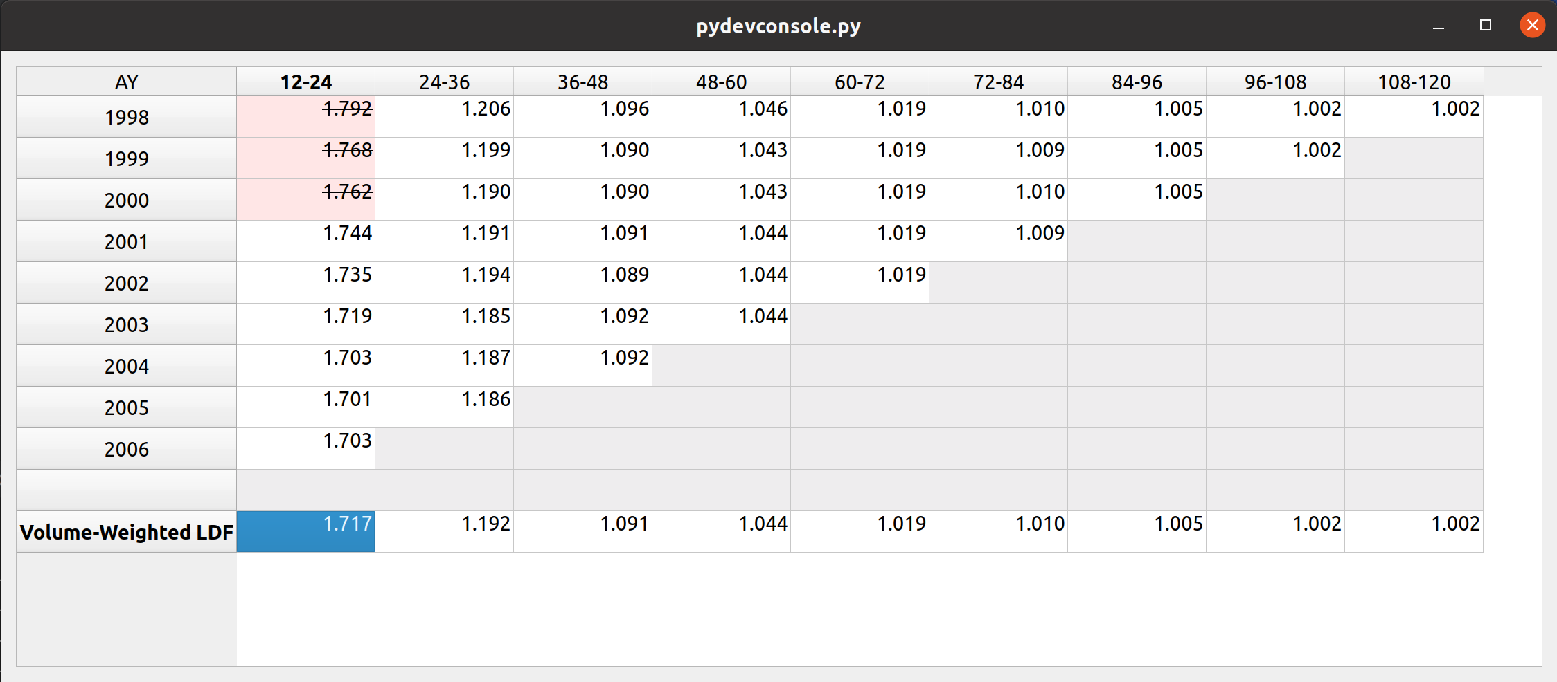
Triangle Preview

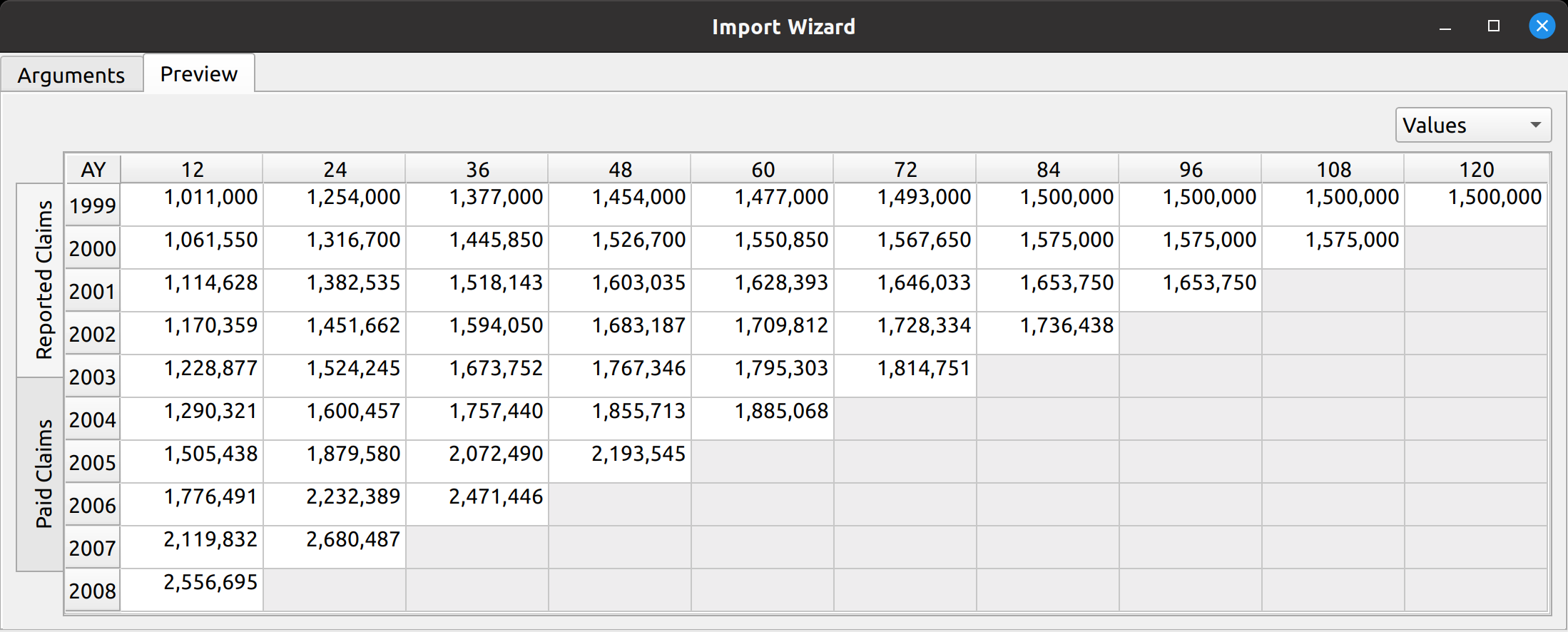
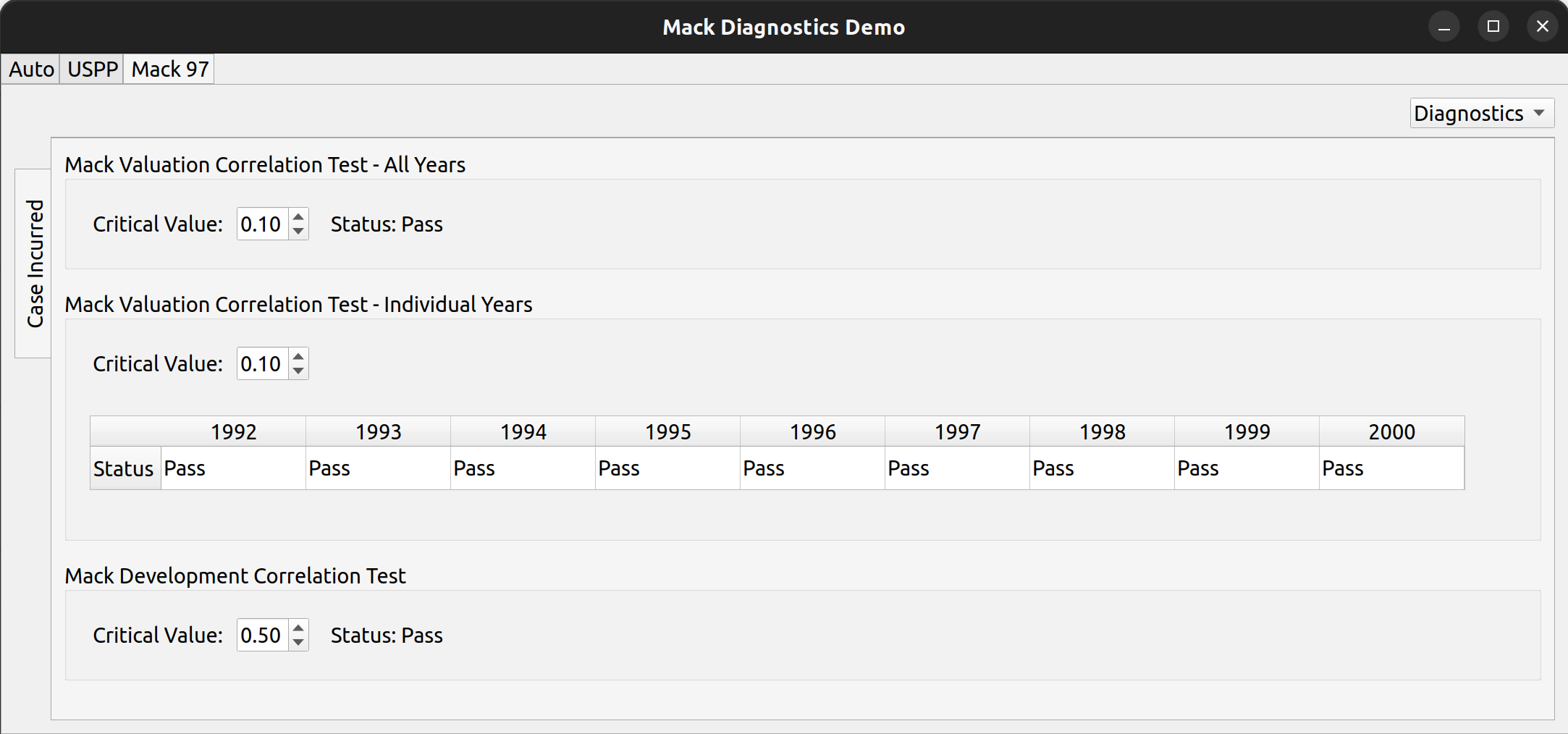
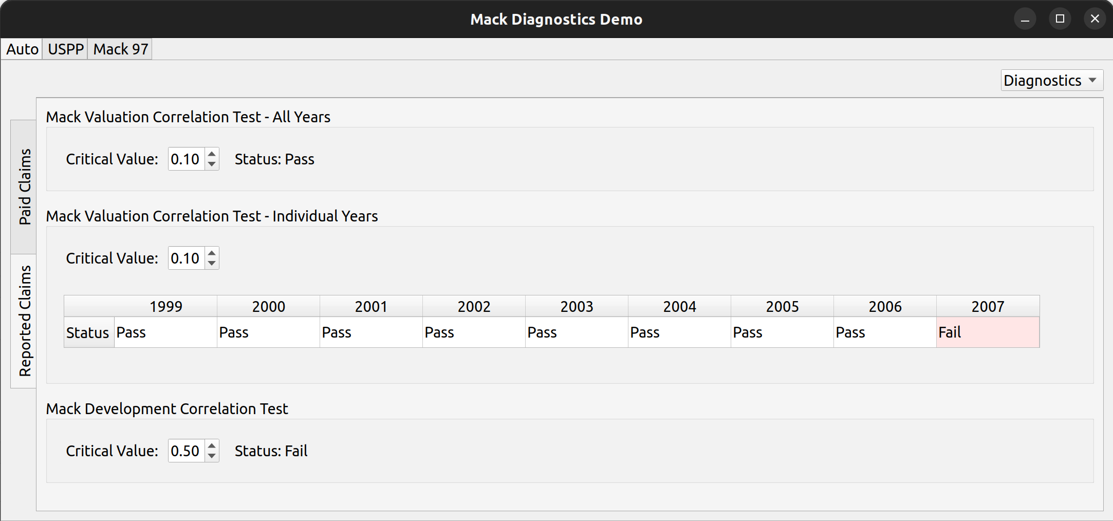
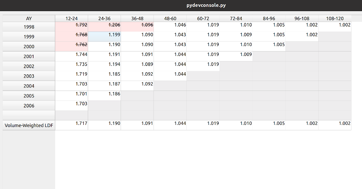
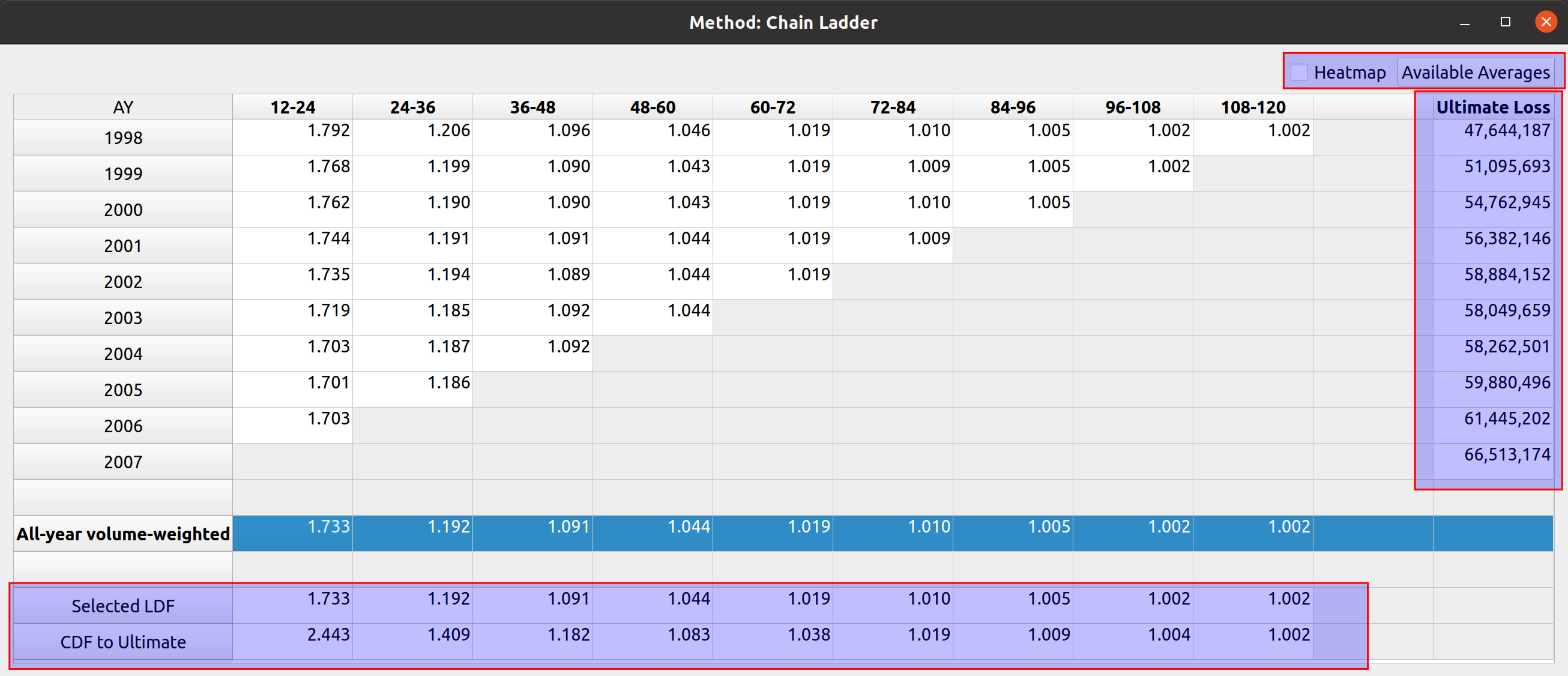
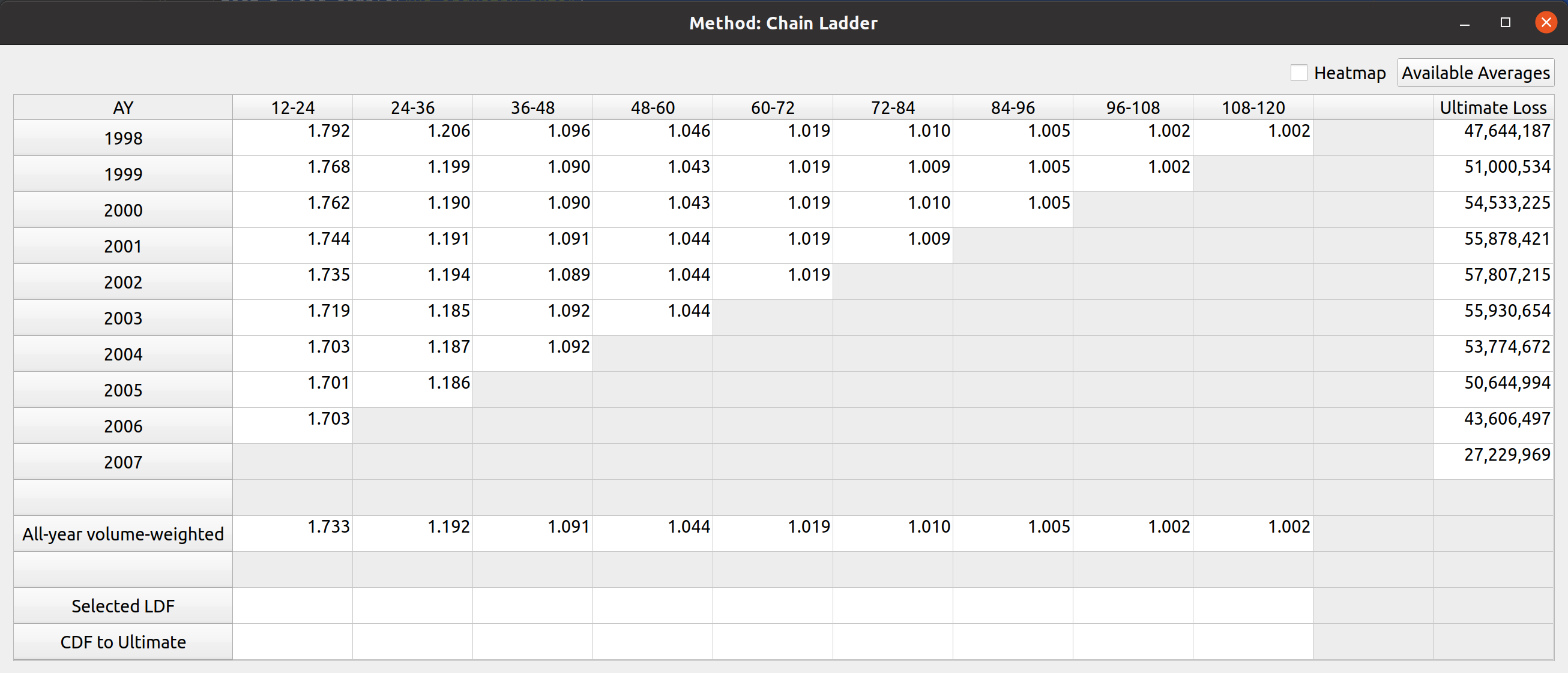
Once the mapping is done, the user can preview the generated triangle by clicking on the “Preview” tab. This tab is populated by the same analysis widget discussed in my last post.

The following video illustrates the entire process in action:

https://genedan.com/wp-content/uploads/2022/10/Screencast-from-10-23-2022-070846-PM.webm

PyQt6 Transition

Another thing that happened since the last release is that FASLR has now been upgraded from PyQt5 to PyQt6. Qt6 has been around for some time, so the transition was planned last year to happen in October of this year once all the features from Qt5 became available. There were some hiccups, but overall the process went smoothly. I have another post planned to discuss it.

Posted in: Actuarial

No. 148: FASLR – Mack Chain Ladder Diagnostics

9 October, 2022 8:22 PM / Leave a Comment / Gene Dan

Today marks an exciting new milestone with the release of FASLR v0.0.2. FASLR (Free Actuarial System for Loss Reserving), is an open-source frontend for loss reserving packages, such as the chainladder package on the Casualty Actuarial Society’s GitHub. As far as I can tell, it’s the first system of its kind – one that will give the actuary full insight into the loss reserving process, from data ingestion to final-sign off, with all the calculations being fully transparent since the source code is freely available.

Last time, I demonstrated that FASLR was able to conduct the most basic loss reserving method, the chain ladder technique. Today I’d like to walk you though some important improvements, the first of which adds new ways to view and arrange triangle data within the program, and the other, which enhances FASLR with diagnostic techniques used to test the assumptions of the chain ladder method.

New features added in v.0.0.2:

  • Analysis pane for viewing different cuts of triangle data
  • Mack diagnostic tests
    • Valuation correlation test across all periods
    • Valuation correlation test for individual periods
    • Development correlation test

The Analysis Pane

The analysis pane is a widget that allows users to view triangle data for multiple lines of business, and within each line of business, to view multiple types of loss statistics, such as paid losses, incurred losses, case reserves etc. Furthermore, the user may choose to toggle between the values themselves (e.g., actual loss dollar amounts) or link ratios to be used to select loss development factors. Additionally, diagnostic outputs used to test the suitability of each triangle for the chain ladder technique, are included.

The above image illustrates the places on the pane where the user can toggle between these views. At the top left there are three tabs, each of which represents a separate line of business. The image below shows how you can click on each tab to view the data contained in each LOB:

To the left, the user can click on the vertically-rotated tabs to switch between different types of triangle data, such as reported and paid claims:

And, by using the combo box to the right, the user can toggle between raw triangle data and derived link ratios:

And lastly, the combo box can also be used to view diagnostic tests, the main subject of this post.

Mack Diagnostic Tests

In his 1997 paper, Measuring the Variability of Chain Ladder Reserve Estimates, Thomas Mack describes a set of assumptions underlying the chain ladder technique:

  1. Successive development factors are not correlated
  2. Accident years are independent

He then describes a set of diagnostic tests which can be used to validate these assumptions. The first one is called the development correlation test, which compares the magnitude of link ratios for each development period and then uses Spearman’s rank correlation coefficient to test for the correlation between development periods.

This test is available in the chainladder package via the DevelopmentCorrelation class. The second assumption is tested by classifying each development period’s link ratios as being either above or below the median, and then comparing the relative counts of these classifications for each diagonal to test for calendar year effects – such as changes in case management philosophy or the introduction of a new claims handling system. Such effects are considered violations of the second assumption.

This test across calendar years can be conducted either in total for all years or for each individual year. The test for calendar year effects is available in the chainladder package via the ValuationCorrelation class. The chainladder documentation contains tutorials on how to use these tests prior to conducting the chain ladder technique.

FASLR includes these three tests as part of the analysis pane:

In the above image, each of three tests is conducted against the triangle found in Mack’s 1997 paper, and are consistent its results (note that the years here go past 1997 – the original paper didn’t have the years so I made them up). Each test is bound by a groupbox, containing a spin box that allows the user to select the critical value used in the hypothesis test. Below is an example where two of the tests have failed, using one of the auto data sets in Friedland’s reserving paper:

Posted in: Actuarial

No. 147: The Chain Ladder Method with FASLR

27 March, 2022 4:25 PM / 2 Comments / Gene Dan

Today marks an exciting milestone – FASLR (Free Actuarial System for Loss Reserving) – has now implemented its first reserving technique, the chain ladder method. This makes it a good time to update the version number for the project, so I’ve bumped it from its inception v0.0.0 to v0.0.1. Feel free to check out the source code on the CAS GitHub.

New features added:

  • Ultimate Loss Column calculated via the chain ladder technique
  • Rows for selected LDFs and CDFs
  • The ability to select LDFs by double-clicking averages
  • Dialog box for creating and storing custom link ratio average types
  • Link ratio heatmap

These features have been added to the development factor view of FASLR. The images below show a comparison to how it looked last month (first image) vs. how it looks now, with the new features highlighted in red boxes (second image):

The FASLR development view, last month.

The FASLR development view, newest version.

Project Status

When examining the views of the repo, I’ve seen a lot of people taking a look at the releases section, the setup.py file, and the documentation. This leads me to believe that some people either think this is an installable program or are checking to see if it is. Right now, the project exists as a collection of Python source code files, so it’s not there yet. I do have plans to eventually release installable binaries where you can just double click a file and have it installed on your operating system. But first, I would have to learn how to do that and I have yet to decide on which tool I want to use to make that happen (GNU Make, Bazel, fbs, pyinstaller, etc.). This will be a new skill for me to acquire so it will take some time.

If you do want to run FASLR, you can execute the file main.py in the shell. This will give you access to the main GUI window and project pane. Currently, I’m focused on setting up views for the various reserving methodologies, once I’ve either exhausted those available in the chainladder package, or reached a point where it would be nice to integrate them into the main window, I will begin to focus more on the reserving project methodology – i.e., making it possible to start from data importation and end with a reserving estimate.

Versioning Methodology

The versioning system consists of a three-part format: v#.#.#. The rightmost digit represents unstable versions. Excluding v0.0.0, if your installation happens to have a rightmost digit other than 0, you can assume that you are using the software for the purpose of testing out the latest features and not relying on stability. The middle digit represents stable releases, meaning that the features have been tested to the best of the ability of the developer(s) and provide a reasonable level of reliability. So something like v0.1.0 would represent the first stable version and v0.1.1 would represent the most recent unstable version released after v0.1.0. The next stable version after v0.1.0 will be v0.2.0.

The leftmost digit represents major cultural milestones in the project. Right now it seems to be in vogue to reserve version 1.whatever for a special occasion, to mark the point where the software has become the de-facto open-source standard for performing work in the field. I will adopt this convention for this project, but while I have no plans to ever reach this point, as FASLR is mostly a learning exercise for me, it would be a nice point to reach if it ever gains traction.

Ultimate Losses

Since there are numerous sources on actuarial reserving methods which can do a much better job of explaining how they work than I can, I won’t spend much detail here on them and you can always refer back to CAS Exam 5 papers if you are not familiar with them. These next few sections will start with a blank factor view, and I will gradually demonstrate how link ratio averages can be used, in combination with the chain ladder technique to project ultimate loss.

One purpose of actuarial reserving is to estimate the liabilities per unit of time (such as accident year) and we call this estimate the ultimate loss. Therefore, one of my goals for this month was to add a column for ultimate loss. Below shows the (mostly) blank factor view with the link ratio triangle and ultimate loss column to the right. The LDFs have not been selected, and the chainladder package defaults non-selection to 1.000:

You can confirm that the starting LDFs are 1.000 by looking at the source triangle – the ultimate loss values are the same as the latest diagonal:

LDF Selection

Below the triangle, you will find a section that has various link ratio averages that you can select by double-clicking on them. The image in the previous section only had one option, the all-year volume-weighted average, but you can add more by selecting the “Available Averages” button in the upper-right hand corner. Doing so will open up a dialog box with averages that you can add to the factor view:

The starting averages are All, 5-, and 3- year volume-weighted averages. You can add these by clicking the checkboxes in the table. Alternatively, you can add a custom type if you want to use a different kind of average like straight or regression. You can do this by clicking the “Add Average” button and then selecting the options for the new average. Right now, only these three are supported by chainladder, but I have proposed that we add others like medial and geometric to the list:

In this example I have added a 2-year regression and selected all 4 average types in the table. This expands the number of rows in the LDF section of the factor view:

Next, you can select the LDFs by double-clicking on the LDF section. Double-clicking an entire row will select that whole row, and the CDFs are automatically calculated. The image below shows that I have selected the 2-year regression, and the ultimate loss values are automatically updated:

Alternatively, you can enter in your own custom values by typing or copy-pasting into the cells directly. And you can delete the selections by pressing the delete key over the cells or by double-clicking the row header of the selected LDF row. You can also remove LDF average types by clicking on the “available averages” button and unchecking the ones you want to remove.

Heatmap

This last feature is something that comes from the chainladder package. It was quite challenging to implement even though on the surface, all you have to do is tick the checkbox. This helps you identify outlier link ratios that you may want to exclude in your analysis:

There are some performance enhancements to be made on this feature, I’ll write up another post once that’s done. Below, you’ll see a gif of all of what I described above in action:

Posted in: Actuarial

No. 146: Development Factors with FASLR

21 February, 2022 5:42 PM / Leave a Comment / Gene Dan

A few things have happened since this last time I’ve posted about a technical subject – I have gotten into contact with Brian Fannin over at the CAS and now have two projects hosted on their GitHub page – PCDM, which I wrote about a couple years ago, and FASLR, a new project I started last year, which I’ll be talking about today.

FASLR (pronounced fæzlɹ̩), is a GUI wrapper built using the PyQt framework to accommodate open-source actuarial reserving engines, such as the chainladder packages written in Python and R.

OK. The buzzword-free version of that sentence is that FASLR is open-source software that is intended to help actuaries do reserving with buttons, windows, and mouse clicks. There are a few open-source packages that let actuaries do reserving by writing programs, and some commercial solutions that let actuaries do reserving with buttons and mouse clicks. But at least to my knowledge, there had yet to be an open-source interface-based software for doing reserving, so I decided to make one. What motivated me to start was I have been wanting to build graphical interfaces for my other projects, such as MIES, but hadn’t made a decision whether to use web-based technologies like Django (letting people use the software in the browser) or something desktop-based like PyQt. I have decided on using PyQt since that would require me to learn fewer languages or deal with browser stuff like JavaScript.

FASLR stands for Free Actuarial System for Loss Reserving, named after Fazlur Rahman Khan, an architect who designed a number of famous buildings in Chicago.

Other motivations include:

  • Giving me an excuse to learn PyQt
  • Increasing transparency on how actuarial computations are done
  • Giving students a window into how actuarial work is done in practice as opposed to exams
  • Increasing accessibility of actuarial software to the general public
  • Making a GUI compatible with existing open-source technologies
  • Imposing my worldview on how actuarial models should be built and implemented in the workplace
  • Bragging rights on the CAS GitHub page
FASLR basic interface

FASLR basic interface

The Chainladder Packages

Chainladder is a fancy word for one of the techniques that actuaries use to guess how much money insurance companies need to pay for claims. It’s also the name of a pair of open-source actuarial packages – one written in R, and another in Python. The R library was written many years ago by Markus Gesmann. It seems to have been written starting around 2007, which is the year of the earliest release I have been able to find on CRAN. The Python package is a port of the R library, written by John S Bogaardt starting around 2017 or so based on the commit history. These packages, by being open-source, have not only helped to improve transparency to how actuarial computations are done but have also improved accessibility to the field by being available to people who do not have the means to pay for commercial software, such as students looking to get into the field. However, since they are lightweight libraries, actuaries must write programs to do reserving – which, depending on personal preference, may or may not be the most productive way to get reserving done.

I think that last sentence is a fair criticism of using a programming language to get actuarial work done – especially when we consider the selection of development factors, the topic of today’s post. This isn’t to disparage these packages – both of which are major contributions to modernizing actuarial science. And thanks to John, pretty much 75% of the work is already done to get FASLR working – all I have to do is design the interface (unlike MIES, which will take forever to be ready). It is their work that makes something like FASLR possible. On the subject of development factors – this is a family of various averages of age-to-age factors used to develop losses to ultimate. When you use a package, you might need to write a line of code picking out which link ratios you want to exclude and then visualize the resulting averages by executing another line. If you didn’t like your selection, you may have to edit that line of code or write a new one and recompute – over and over again. That may be tedious, and hard to keep track of if you have several attempts. However, if you could simply double-click on a triangle of link ratios to exclude them and see the factors update in near-real time, you can get your work done a lot faster.

Below is an example (taken from the Chainladder documentation) of how we can use Chainladder to load a sample triangle and see the link ratios:

Python
1
2
3
4
5
import chainladder as cl
 
genins = cl.load_sample("genins")
 
print(genins.link_ratio)

1
2
3
4
5
6
7
8
9
10
         12-24     24-36     36-48     48-60     60-72     72-84     84-96    96-108   108-120
2001  3.143200  1.542806  1.278299  1.237719  1.209207  1.044079  1.040374  1.063009  1.017725
2002  3.510582  1.755493  1.545286  1.132926  1.084493  1.128106  1.057268  1.086496       NaN
2003  4.448450  1.716718  1.458257  1.232079  1.036860  1.120010  1.060577       NaN       NaN
2004  4.568002  1.547052  1.711784  1.072518  1.087360  1.047076       NaN       NaN       NaN
2005  2.564198  1.872956  1.361545  1.174217  1.138315       NaN       NaN       NaN       NaN
2006  3.365588  1.635679  1.369162  1.236443       NaN       NaN       NaN       NaN       NaN
2007  2.922798  1.878099  1.439393       NaN       NaN       NaN       NaN       NaN       NaN
2008  3.953288  2.015651       NaN       NaN       NaN       NaN       NaN       NaN       NaN
2009  3.619179       NaN       NaN       NaN       NaN       NaN       NaN       NaN       NaN

And to view the volume-weighted LDFs for all years, we execute:

Python
1
2
3
vol = cl.Development(average="volume").fit(genins).ldf_
 
print(vol)

1
2
          12-24     24-36     36-48     48-60     60-72     72-84     84-96    96-108   108-120
(All)  3.490607  1.747333  1.457413  1.173852  1.103824  1.086269  1.053874  1.076555  1.017725

Now, to exclude certain periods, we can pass a list of excluded periods to the .Development() method:

1
2
3
ldfs_w_dropped = cl.Development(drop=[("2004", 12), ("2008", 24)]).fit(genins).ldf_
 
print(ldfs_w_dropped)

1
2
          12-24     24-36     36-48     48-60     60-72     72-84     84-96    96-108   108-120
(All)  3.379677  1.704149  1.457413  1.173852  1.103824  1.086269  1.053874  1.076555  1.017725

We can see that this has altered the 12-24 and 24-36 LDFs.

However, actuaries typically want to experiment with several exclusions with trial and error, so a GUI would be helpful here.

FASLR Example

I will now give a demo of how FASLR uses the Chainladder methods above to speed up LDF selection via a GUI. Below is an example of a window I designed to display a triangle of link ratios with the volume-weighted LDFs right below the triangle:

What I’d like to do is double-click a factor to exclude it. Ideally this will get the LDFs at the bottom to update immediately so I can see the results – without having to do all the typing we did with the Chainladder example. I have written FASLR to update the formatting of the link ratio to be struck-out with a pink background to indicate exclusion. Below are the first three accident years of the 12-24 column excluded.

You can see that the formatting has now updated with the first ldf changed from 1.733 to 1.717.

The GIF below demonstrates how fast we can preview the LDF changes using this feature:

The demo can be run from the FASLR source code, available on the CAS GitHub page.

This is just one feature preview out of what I hope will be many, so keep an eye open for future updates.

Technical Appendix

This was all much easier said than done. Getting that factor elimination feature to work was tricky, especially with me being new to PyQt and all. This feature makes use of a concept called Model-View-Controller which you can read more about here. Below is some example code from the FASLR module that does most of the work that we see in today’s post. It depends on all the other modules in the repository, so I don’t expect a full understanding from the code listing alone. To find out more, refer to the entire source code:

Python
1
2
3
4
5
6
7
8
9
10
11
12
13
14
15
16
17
18
19
20
21
22
23
24
25
26
27
28
29
30
31
32
33
34
35
36
37
38
39
40
41
42
43
44
45
46
47
48
49
50
51
52
53
54
55
56
57
58
59
60
61
62
63
64
65
66
67
68
69
70
71
72
73
74
75
76
77
78
79
80
81
82
83
84
85
86
87
88
89
90
91
92
93
94
95
96
97
98
99
100
101
102
103
104
105
106
107
108
109
110
111
112
113
114
115
116
117
118
119
120
121
122
123
124
125
126
127
128
129
130
131
132
133
134
135
136
137
138
139
140
141
142
143
144
145
146
147
148
149
150
151
152
153
154
155
156
157
158
159
160
161
162
163
164
165
166
167
168
169
170
171
172
173
174
175
176
177
178
179
180
181
182
183
184
185
186
187
188
189
190
191
192
193
194
195
196
197
198
199
200
201
202
203
204
205
206
207
208
209
210
211
212
213
214
215
216
217
218
219
220
221
222
223
224
225
226
227
228
229
230
231
232
233
234
235
236
237
238
239
240
241
242
243
244
245
246
247
248
249
250
251
252
253
254
255
256
257
258
259
260
261
262
263
264
265
266
267
268
269
270
271
272
273
274
275
276
277
278
279
280
281
282
283
284
285
286
287
288
289
290
291
292
293
294
295
296
297
298
299
300
301
302
303
304
305
306
307
308
309
310
311
312
313
314
315
316
317
318
319
320
321
322
323
324
325
326
327
328
329
330
331
import chainladder as cl
import csv
import io
import numpy as np
import pandas as pd
 
from chainladder import Triangle
 
from pandas import DataFrame
 
from PyQt5.QtCore import (
    QAbstractTableModel,
    QEvent,
    Qt,
    QSize,
    QVariant
)
 
from PyQt5.QtGui import (
    QColor,
    QFont,
    QKeySequence
)
 
from PyQt5.QtWidgets import (
    QAbstractButton,
    QAction,
    QApplication,
    qApp,
    QLabel,
    QMenu,
    QStyle,
    QStylePainter,
    QStyleOptionHeader,
    QTableView,
    QVBoxLayout
)
 
from style.triangle import (
    BLANK_TEXT,
    LOWER_DIAG_COLOR,
    RATIO_STYLE,
    VALUE_STYLE
)
 
 
class FactorModel(QAbstractTableModel):
 
    def __init__(
            self,
            triangle: Triangle,
            value_type: str = "ratio"
    ):
        super(
            FactorModel,
            self
        ).__init__()
 
        self.triangle = triangle
        self._data = triangle.link_ratio.to_frame()
        self.link_frame = triangle.link_ratio.to_frame()
        self.n_rows = self.rowCount()
 
        self.development_factors = cl.Development(average="volume").fit(self.triangle)
 
        self._data = get_display_data(
            ratios=self.link_frame,
            factors=self.development_factors
        )
 
        self.value_type = value_type
        self.excl_frame = self._data.copy()
        self.excl_frame.loc[:] = False
        self.blank_row_num = self.n_rows + 1
 
    def data(
            self,
            index,
            role=None
    ):
 
        if role == Qt.DisplayRole:
 
            value = self._data.iloc[index.row(), index.column()]
 
            # Display blank when there are nans in the lower-right hand of the triangle.
            if str(value) == "nan":
 
                display_value = BLANK_TEXT
            else:
                # "value" means stuff like losses and premiums, should have 2 decimal places.
                if self.value_type == "value":
 
                    display_value = VALUE_STYLE.format(value)
 
                # for "ratio", want to display 3 decimal places.
                else:
 
                    display_value = RATIO_STYLE.format(value)
 
                display_value = str(display_value)
 
            self.setData(
                self.index(
                    index.row(),
                    index.column()
                ),
                QVariant(Qt.AlignRight),
                Qt.TextAlignmentRole
            )
 
            return display_value
 
        if role == Qt.TextAlignmentRole:
            return Qt.AlignRight
 
        if role == Qt.BackgroundRole:
            if (index.column() >= self.n_rows - index.row()) and \
                    (index.row() < self.blank_row_num):
                return LOWER_DIAG_COLOR
            elif index.row() < self.blank_row_num:
                exclude = self.excl_frame.iloc[[index.row()], [index.column()]].squeeze()
 
                if exclude:
                    return QColor(255, 230, 230)
                else:
                    return QColor(255, 255, 255)
        if (role == Qt.FontRole) and (self.value_type == "ratio") and (index.row() < self.blank_row_num):
            font = QFont()
            exclude = self.excl_frame.iloc[[index.row()], [index.column()]].squeeze()
            if exclude:
                font.setStrikeOut(True)
            else:
                font.setStrikeOut(False)
            return font
 
    def rowCount(
            self,
            parent=None,
            *args,
            **kwargs
    ):
 
        return self._data.shape[0]
 
    def columnCount(
            self,
            parent=None,
            *args,
            **kwargs
    ):
 
        return self._data.shape[1]
 
    def headerData(
            self,
            p_int,
            qt_orientation,
            role=None
    ):
 
        # section is the index of the column/row.
        if role == Qt.DisplayRole:
            if qt_orientation == Qt.Horizontal:
                return str(self._data.columns[p_int])
 
            if qt_orientation == Qt.Vertical:
                return str(self._data.index[p_int])
 
    def toggle_exclude(self, index):
        exclude = self.excl_frame.iloc[[index.row()], [index.column()]].squeeze()
 
        if exclude:
            self.excl_frame.iloc[[index.row()], [index.column()]] = False
        else:
            self.excl_frame.iloc[[index.row()], [index.column()]] = True
 
    def recalculate_factors(self, index):
 
        drop_list = []
        for i in range(self.link_frame.shape[0]):
            for j in range(self.link_frame.shape[1]):
 
                exclude = self.excl_frame.iloc[[i], [j]].squeeze()
                print(exclude)
 
                if exclude:
 
                    row_drop = str(self.link_frame.iloc[i].name)
                    col_drop = int(str(self.link_frame.columns[j]).split('-')[0])
 
                    drop_list.append((row_drop, col_drop))
 
                else:
 
                    pass
 
        development = cl.Development(drop=drop_list, average="volume")
 
        self.development_factors = development.fit(self.triangle)
        self._data = get_display_data(
            ratios=self.link_frame,
            factors=self.development_factors
        )
 
        # print(development.fit_transform(self.triangle).link_ratio)
 
        print(self._data)
        self.dataChanged.emit(index, index)
        self.layoutChanged.emit()
 
 
class FactorView(QTableView):
    def __init__(self):
        super().__init__()
 
        self.copy_action = QAction("&Copy", self)
        self.copy_action.setShortcut(QKeySequence("Ctrl+c"))
        self.copy_action.setStatusTip("Copy selection to clipboard.")
        # noinspection PyUnresolvedReferences
        self.copy_action.triggered.connect(self.copy_selection)
 
        self.installEventFilter(self)
 
        btn = self.findChild(QAbstractButton)
        btn.installEventFilter(self)
        btn_label = QLabel("AY")
        btn_label.setAlignment(Qt.AlignCenter)
        btn_layout = QVBoxLayout()
        btn_layout.setContentsMargins(0, 0, 0, 0)
        btn_layout.addWidget(btn_label)
        btn.setLayout(btn_layout)
        opt = QStyleOptionHeader()
 
        # Set the styling for the table corner so that it matches the rest of the headers.
        self.setStyleSheet(
            """
            QTableCornerButton::section{
                border-width: 1px;
                border-style: solid;
                border-color:none darkgrey darkgrey none;
            }
            """
        )
 
        s = QSize(btn.style().sizeFromContents(
            QStyle.CT_HeaderSection, opt, QSize(), btn).
                  expandedTo(QApplication.globalStrut()))
 
        if s.isValid():
            self.verticalHeader().setMinimumWidth(s.width())
 
        self.verticalHeader().setDefaultAlignment(Qt.AlignCenter)
 
        self.doubleClicked.connect(self.exclude_ratio)
 
    def exclude_ratio(self):
        selection = self.selectedIndexes()
 
        for index in selection:
            index.model().toggle_exclude(index=index)
            index.model().recalculate_factors(index=index)
 
    def eventFilter(self, obj, event):
        if event.type() != QEvent.Paint or not isinstance(
                obj, QAbstractButton):
            return False
 
        # Paint by hand (borrowed from QTableCornerButton)
        opt = QStyleOptionHeader()
        opt.initFrom(obj)
        style_state = QStyle.State_None
        if obj.isEnabled():
            style_state |= QStyle.State_Enabled
        if obj.isActiveWindow():
            style_state |= QStyle.State_Active
        if obj.isDown():
            style_state |= QStyle.State_Sunken
        opt.state = style_state
        opt.rect = obj.rect()
        # This line is the only difference to QTableCornerButton
        opt.text = obj.text()
        opt.position = QStyleOptionHeader.OnlyOneSection
        painter = QStylePainter(obj)
        painter.drawControl(QStyle.CE_Header, opt)
 
        return True
 
    def contextMenuEvent(self, event):
        """
        When right-clicking a cell, activate context menu.
 
        :param: event
        :return:
        """
        menu = QMenu()
        menu.addAction(self.copy_action)
        menu.exec(event.globalPos())
 
    def copy_selection(self):
        """Method to copy selected values to clipboard, so they can be pasted elsewhere, like Excel."""
        selection = self.selectedIndexes()
        if selection:
            rows = sorted(index.row() for index in selection)
            columns = sorted(index.column() for index in selection)
            rowcount = rows[-1] - rows[0] + 1
            colcount = columns[-1] - columns[0] + 1
            table = [[''] * colcount for _ in range(rowcount)]
            for index in selection:
                row = index.row() - rows[0]
                column = index.column() - columns[0]
                table[row][column] = index.data()
            stream = io.StringIO()
            csv.writer(stream, delimiter='\t').writerows(table)
            qApp.clipboard().setText(stream.getvalue())
        return
 
 
def get_display_data(ratios, factors: DataFrame):
 
    data = {"": [np.nan] * len(ratios.columns)}
 
    blank_row = pd.DataFrame.from_dict(
        data,
        orient="index",
        columns=ratios.columns
    )
 
    factor_frame = factors.ldf_.to_frame()
    factor_frame = factor_frame.rename(index={'(All)': 'Volume-Weighted LDF'})
    return pd.concat([ratios, blank_row, factor_frame])

Posted in: Actuarial

No. 144: MIES – Intertemporal Choice

26 July, 2020 10:11 PM / Leave a Comment / Gene Dan

This entry is part of a series dedicated to MIES – a miniature insurance economic simulator. The source code for the project is available on GitHub.

Current Status

This week, I’ve been continuing my work on incorporating risk into the consumer behavior component of MIES. The next step in this process involves the concept of intertemporal choice, an interpretation of the budget constraint problem whereby a consumer can shift consumption from one time period to another by means of savings and loans. The content of this post follows chapter 10 of Varian.

For example, a person can consume more in a future period by saving money. A person can also increase their consumption today by taking out a loan, which comes at a cost of future consumption because they have to pay interest. When making decisions between current and future consumption, we also have to think about time value of money. When I was reading through Varian, I was happy to see that many of the concepts I learned from the financial mathematics actuarial exam were also discussed by Varian – such as bonds, annuities, and perpetuities – albeit in much less detail.

This inspired me to create a new repo to handle time value of money computations, which is not yet ready for its own series of posts, but for which you can see the initial work here. I had intended to make this repo further out in the future, but I got excited and started early.

Also relevant, is the concept of actuarial communication. Now that I’m blogging more about actuarial work, I will need to be able to write the notation here. There are some \LaTeX packages that can render actuarial notation, such as actuarialsymbol. Actuaries are still in the stone age when it comes to sharing technical work over the Internet, not out of ignorance, since many actuaries are familiar with \LaTeX, but out of corporate inertia in getting the right tools at work (which I can suppose be due to failure to persuade the right people) and lack of momentum and willingness as many people simply just try to make do with using ASCII characters to express mathematical notation. I think this is a major impediment to adding rigor to practical actuarial work, which many young analysts complain about when they first start working, as they notice that spreadsheet models tend to be a lot more dull than what they see on the exams.

I was a bit anxious in trying to get the actuarialsymbol package working since, although I knew how to get it working on my desktop, I wasn’t sure if it would work with WordPress or Anki, a study tool that I use. Fortunately, it does work! For example, the famous annuity symbol can be rendered with the command \ax{x:\angln}:

Rendered by QuickLaTeX.com

That was easy. There’s no reason why intraoffice email can’t support this, so I hope that it encourages you to pick it up as well.

The Statics Module

Up until now, testing new features has been cumbersome since many of the previous demos I have written about required existing simulation data. That is, in order to test things like intertemporal choice, I would first need to set up a simulation, run it, and then use the results as inputs into the new functions, classes, or methods.

That really shouldn’t be necessary, especially since many of the concepts I have been making modules for apply to economics in general, and not just to insurance. To solve this problem, I created the statics module, which is named after the process of comparative statics, which examines how behavior changes when an exogenous variable in the model changes (aka all the charts I’ve been making about MIES).

The statics module currently has one class, Consumption, which can return attributes such as the optimal consumption of a person given a budget and utility function:

Python
1
2
3
4
5
6
7
8
9
10
11
12
13
14
15
16
17
18
19
20
21
22
23
24
25
26
27
28
29
30
31
32
33
34
35
36
37
38
39
40
41
42
43
44
45
46
47
48
49
50
51
52
53
54
55
56
57
58
59
60
61
62
63
64
65
# used for comparative statics
import plotly.graph_objects as go
 
from plotly.offline import plot
 
from econtools.budget import Budget
from econtools.utility import CobbDouglas
 
 
class Consumption:
    def __init__(
            self,
            budget: Budget,
            utility: CobbDouglas
    ):
        self.budget = budget
        self.income = self.budget.income
        self.utility = utility
        self.optimal_bundle = self.get_consumption()
        self.fig = self.get_consumption_figure()
 
    def get_consumption(self):
        optimal_bundle = self.utility.optimal_bundle(
            p1=self.budget.good_x.adjusted_price,
            p2=self.budget.good_y.adjusted_price,
            m=self.budget.income
        )
 
        return optimal_bundle
 
    def get_consumption_figure(self):
        fig = go.Figure()
        fig.add_trace(self.budget.get_line())
        fig.add_trace(self.utility.trace(
            k=self.optimal_bundle[2],
            m=self.income / self.budget.good_x.adjusted_price * 1.5
        ))
 
        fig.add_trace(self.utility.trace(
            k=self.optimal_bundle[2] * 1.5,
            m=self.income / self.budget.good_x.adjusted_price * 1.5
        ))
 
        fig.add_trace(self.utility.trace(
            k=self.optimal_bundle[2] * .5,
            m=self.income / self.budget.good_x.adjusted_price * 1.5
        ))
 
        fig['layout'].update({
            'title': 'Consumption',
            'title_x': 0.5,
            'xaxis': {
                'title': 'Amount of ' + self.budget.good_x.name,
                'range': [0, self.income / self.budget.good_x.adjusted_price * 1.5]
            },
            'yaxis': {
                'title': 'Amount of ' + self.budget.good_y.name,
                'range': [0, self.income * 1.5]
            }
        })
 
        return fig
 
    def show_consumption(self):
        plot(self.fig)

A lot of the code here is the same as that which can be found in the Person class. However, instead of needing to instantiate a person to do comparative statics, I can just use the Consumption class directly from the statics module. This should make creating and testing examples much easier.

Since much of the code in statics is the same as in the Person class, that gives me a hint that I can make things more maintainable by refactoring the code. I would think the right thing to do is to have the Person class use the Consumption class in the statics module, rather than the other way around.

The Intertemporal Class

The intertemporal budget constraint is:

    \[c_1 + c_2/(1+r) = m_1 + m_2/(1+r)\]

Note that this has the same form as the endowment budget constraint:

    \[p_1 x_1 + p_2 x_2 = p_1 m_1 + p_2 m_2 \]

With the difference being that the two endowment goods are now replaced by consumption in times 1 and 2, represented by the cs and the prices, the ps are now replaced by discounted unit prices. The subscript 1 represents the current time and the subscript 2 represents the future time, with the price of future consumption being discounted to present value via the interest rate, r.

The consumer can shift consumption between periods 1 and 2 via saving and lending, subject to the constraint that the amount saved during the first period cannot exceed their first period income, and the amount borrowed during the first period cannot exceed the present value of the income of the second period.

Since the intertemporal budget constraint is a form of the endowment constraint, we can modify the Endowment class in MIES to accommodate this type of consumption. I have created a subclass called Intertemporal that inherits from the Endowment class:

Python
1
2
3
4
5
6
7
8
9
10
11
12
13
14
15
16
17
18
19
20
21
class Intertemporal(Endowment):
    def __init__(
            self,
            good_x: Good,
            good_y: Good,
            good_x_quantity: float,
            good_y_quantity: float,
            interest_rate: float = 0,
            inflation_rate: float = 0
            ):
        Endowment.__init__(
            self,
            good_x,
            good_y,
            good_x_quantity,
            good_y_quantity,
        )
        self.interest_rate = interest_rate
        self.inflation_rate = inflation_rate
        self.good_y.interest_rate = self.interest_rate
        self.good_y.inflation_rate = self.inflation_rate

The main difference here is that the Intertemporal class can accept an interest rate and an inflation rate to adjust the present value of future consumption.

Example

As an example, suppose we have a person who makes 5 dollars in each of time periods 1 and 2. The market interest rate is 10% and their utility function takes the Cobb Douglas form of:

    \[u(x_1, x_2) = x_1^{.5} x_2^{.5}\]

which means they will spend half of the present value of the endowment as consumption in period 1:

Python
1
2
3
4
5
6
7
8
9
10
11
12
13
14
15
16
17
18
19
20
21
22
23
24
from econtools.budget import Budget, Intertemporal, Good
from econtools.statics import Consumption
from econtools.utility import CobbDouglas
 
# test if intercepts plot appropriately with an interest rate of 10%
m1 = Good(price=1, name='Time 1 Consumption')
 
m2 = Good(price=1, name='Time 2 Consumption')
 
endowment = Intertemporal(
    good_x=m1,
    good_y=m2,
    good_x_quantity=5,
    good_y_quantity=5,
    interest_rate=.10
)
 
budget = Budget.from_endowment(endowment, name='budget')
 
utility = CobbDouglas(.5, 0.5)
 
consumption = Consumption(budget=budget, utility=utility)
 
consumption.show_consumption()

The main thing that sticks out here is that the slope of the budget constraint has changed to reflect the adjustment of income to present value. The x-axis intercept is slightly less than 10 because the present value of income is slightly less than 10, and the y-axis intercept is slightly more than 10 because if a person saved all of their time 1 income, they would receive interest of 5 * .1 = .5, making maximum consumption in period 2 10.5.

Since the person allocates half of the present value of the endowment to time 1 consumption, this means they will spend (5 + 5/1.1) * .5 = 4.77 in period one, saving 5 – 4.77 = .23, which then grows to .23 * (1 + .1) = .25 in period 2, which allows for a time 2 consumption of 5 + .25 = 5.25. This is verified by calling the optimal_bundle() method of the Consumption class:

Python
1
2
consumption.optimal_bundle
Out[7]: (4.7727272727272725, 5.25, 5.005678593539359)

Further Improvements

The Varian chapter on intertemporal choice briefly explores present value calculations for various payment streams, such as bonds and perpetuities. I first made a small attempt at creating a tvm module, but quickly realized that the subject of time value of money is much more complex than what is introduced in Varian, since I know that other texts go further in depth, and hence it may be necessary to split a new repo off from MIES so that it can be distributed separately. This repo is called TmVal, the early stages of which I have uploaded here.

Neither of these are ready for demonstration, but you can click on the links if you are interested in seeing what I have done. The next chapter of Varian covers asset markets, which at first glance seems to just be some examples of economic models, so I’m not sure if it has any features I would like to add to MIES. There is still more work to be done on refactoring the code, so I may do that, or move further into risk aversion, or do some more work on TmVal.

Posted in: Actuarial, MIES / Tagged: economics, insurance, intertemporal choice, MIES

Post Navigation

« Previous 1 2 3 4 Next »

Archives

  • August 2025
  • July 2025
  • September 2023
  • February 2023
  • January 2023
  • October 2022
  • March 2022
  • February 2022
  • December 2021
  • July 2020
  • June 2020
  • May 2020
  • May 2019
  • April 2019
  • November 2018
  • September 2018
  • August 2018
  • December 2017
  • July 2017
  • March 2017
  • November 2016
  • December 2014
  • November 2014
  • October 2014
  • August 2014
  • July 2014
  • June 2014
  • February 2014
  • December 2013
  • October 2013
  • August 2013
  • July 2013
  • June 2013
  • March 2013
  • January 2013
  • November 2012
  • October 2012
  • September 2012
  • August 2012
  • July 2012
  • June 2012
  • May 2012
  • April 2012
  • March 2012
  • February 2012
  • January 2012
  • December 2011
  • September 2011
  • August 2011
  • July 2011
  • June 2011
  • January 2011
  • December 2010
  • October 2010
  • September 2010
  • August 2010
  • June 2010
  • May 2010
  • April 2010
  • March 2010
  • September 2009
  • August 2009
  • May 2009
  • December 2008

Categories

  • Actuarial
  • Cycling
  • FASLR
  • Logs
  • Mathematics
  • MIES
  • Music
  • Uncategorized

Links

Cyclingnews
Jason Lee
Knitted Together
Megan Turley
Shama Cycles
Shama Cycles Blog
South Central Collegiate Cycling Conference
Texas Bicycle Racing Association
Texbiker.net
Tiffany Chan
USA Cycling
VeloNews

Texas Cycling

Cameron Lindsay
Jacob Dodson
Ken Day
Texas Cycling
Texas Cycling Blog
Whitney Schultz
© Copyright 2026 - Gene Dan's Blog
Infinity Theme by DesignCoral / WordPress