This entry is part of a series dedicated to MIES – a miniature insurance economic simulator. The source code for the project is available on GitHub.
Current Status
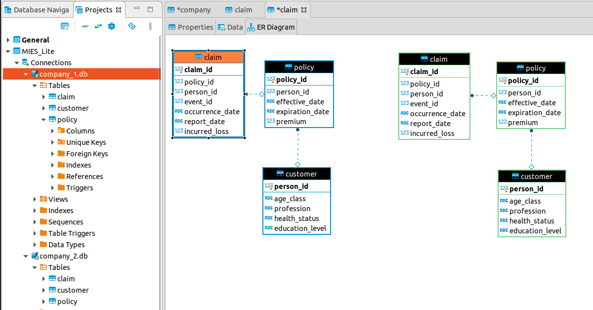
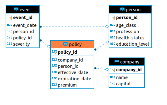
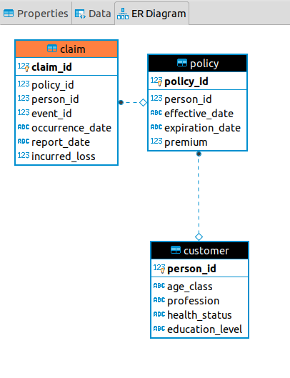
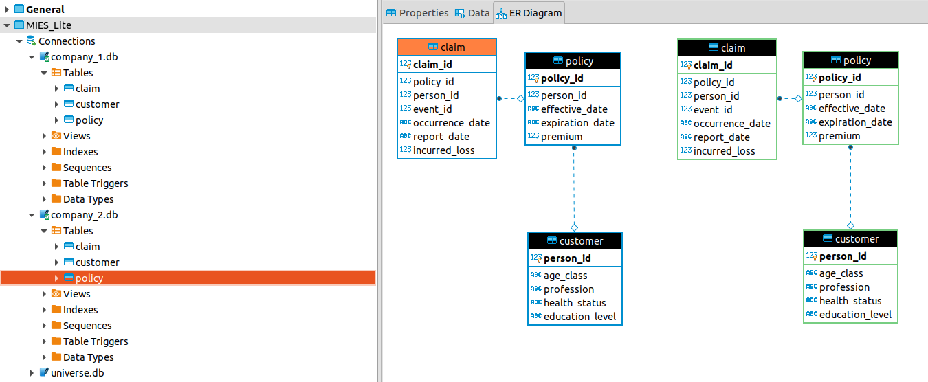
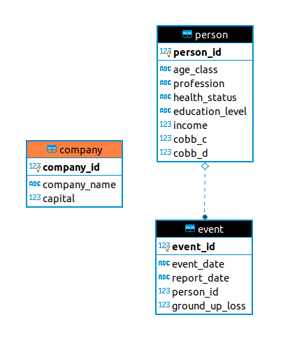
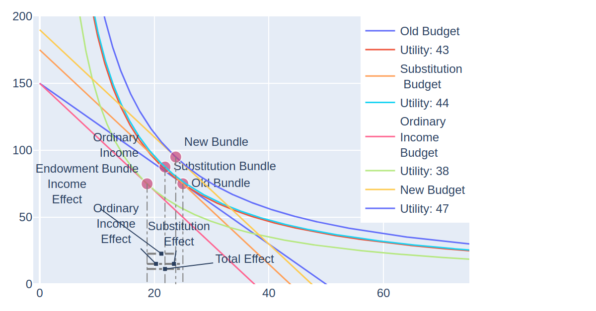
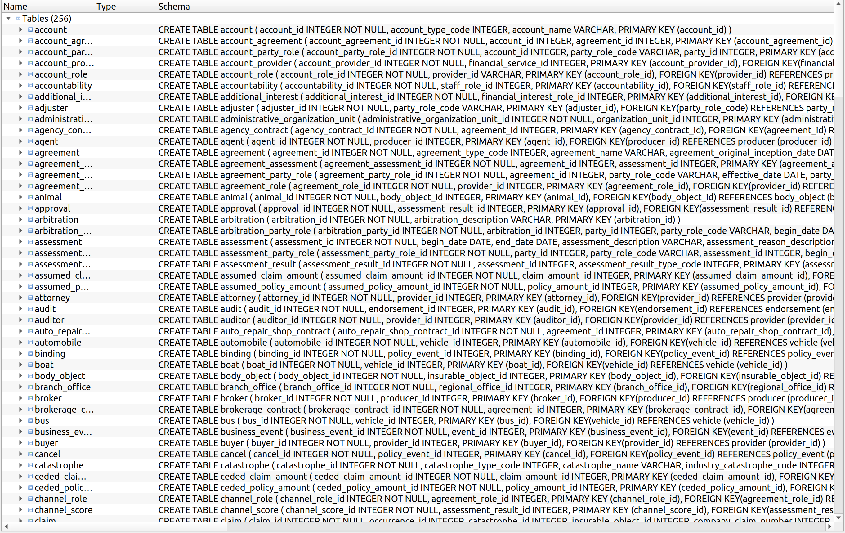
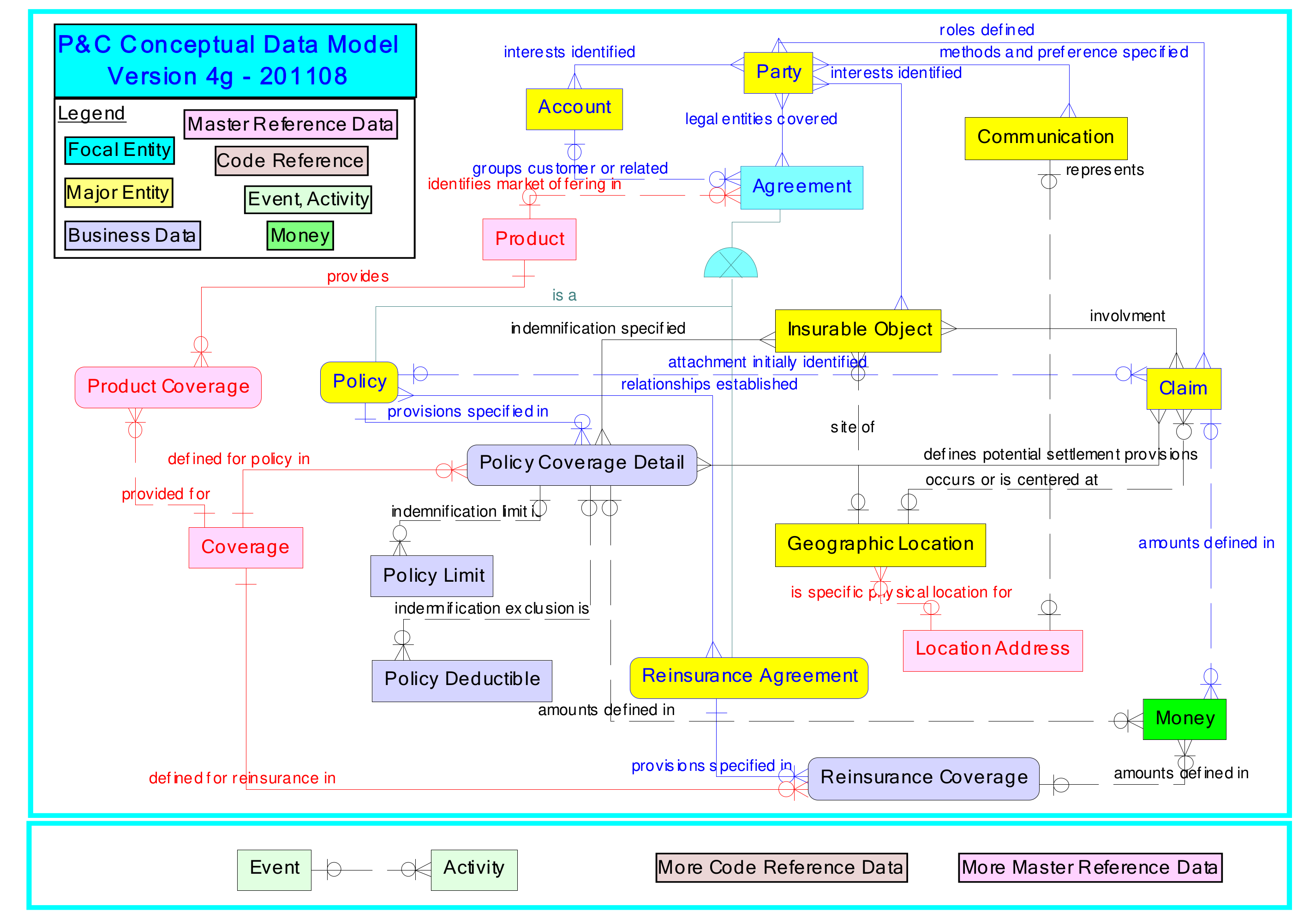
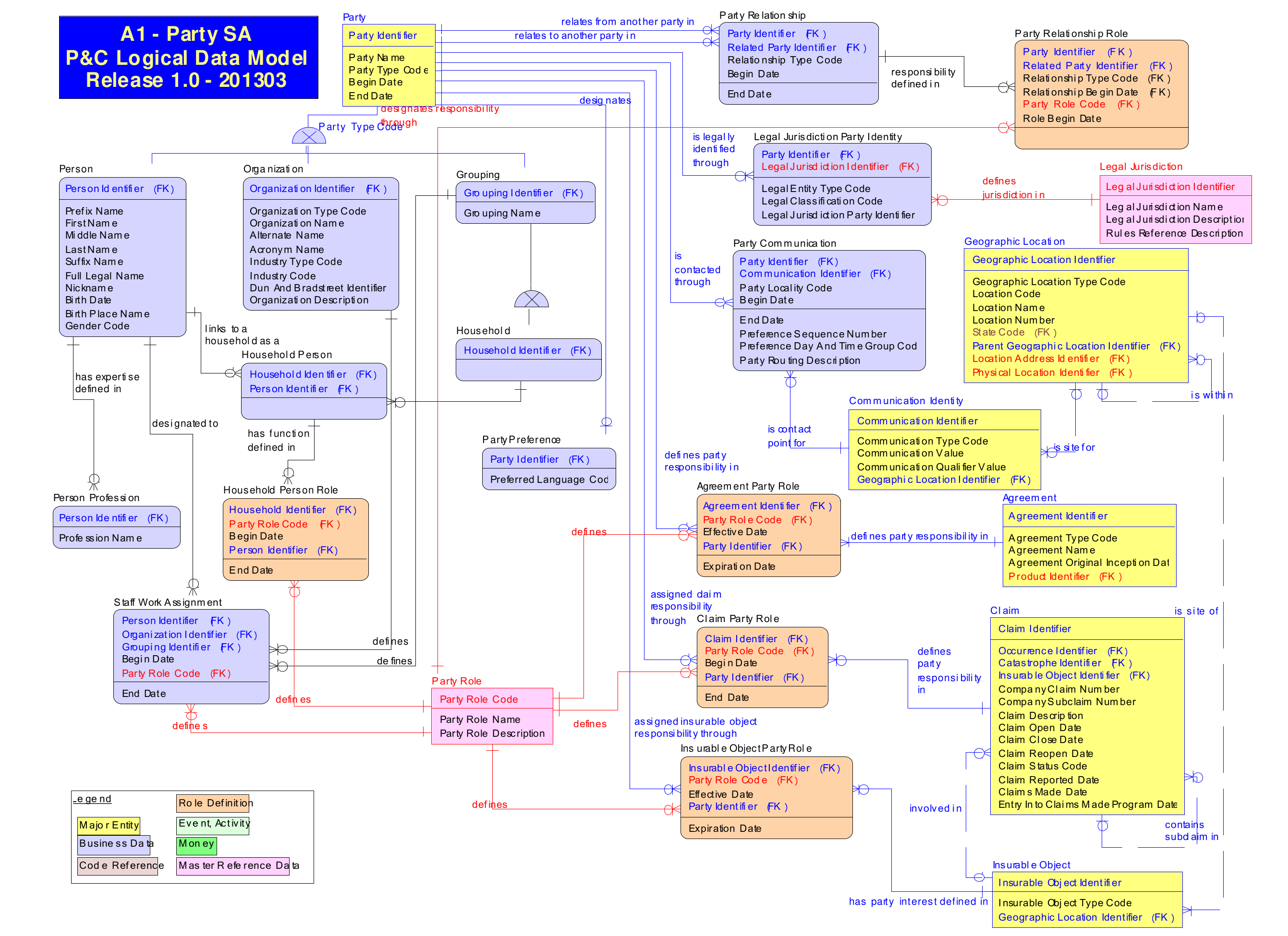
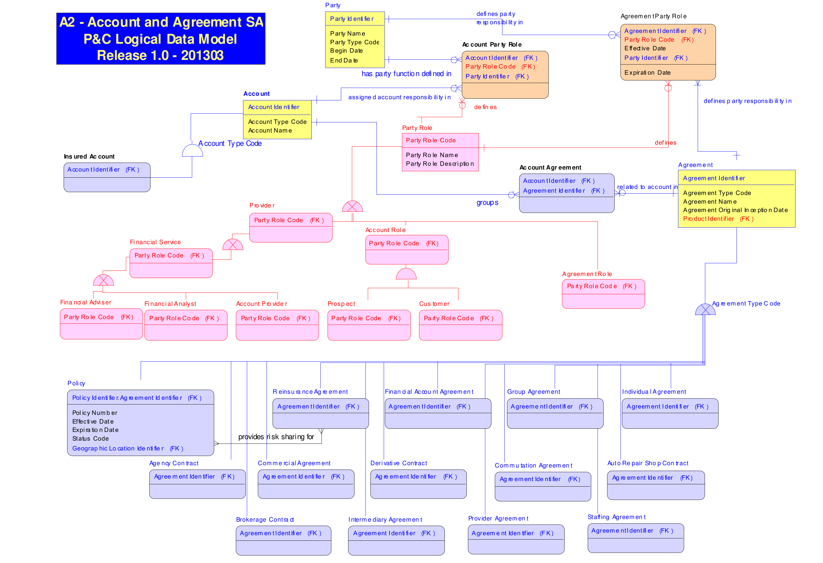
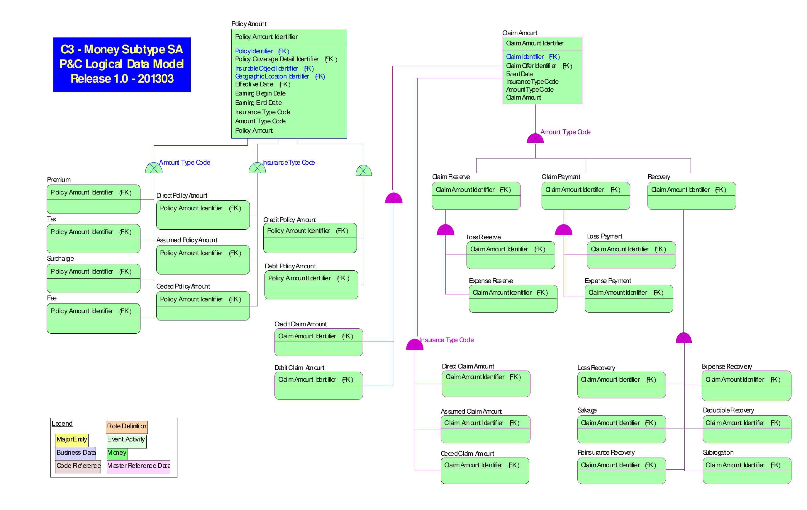
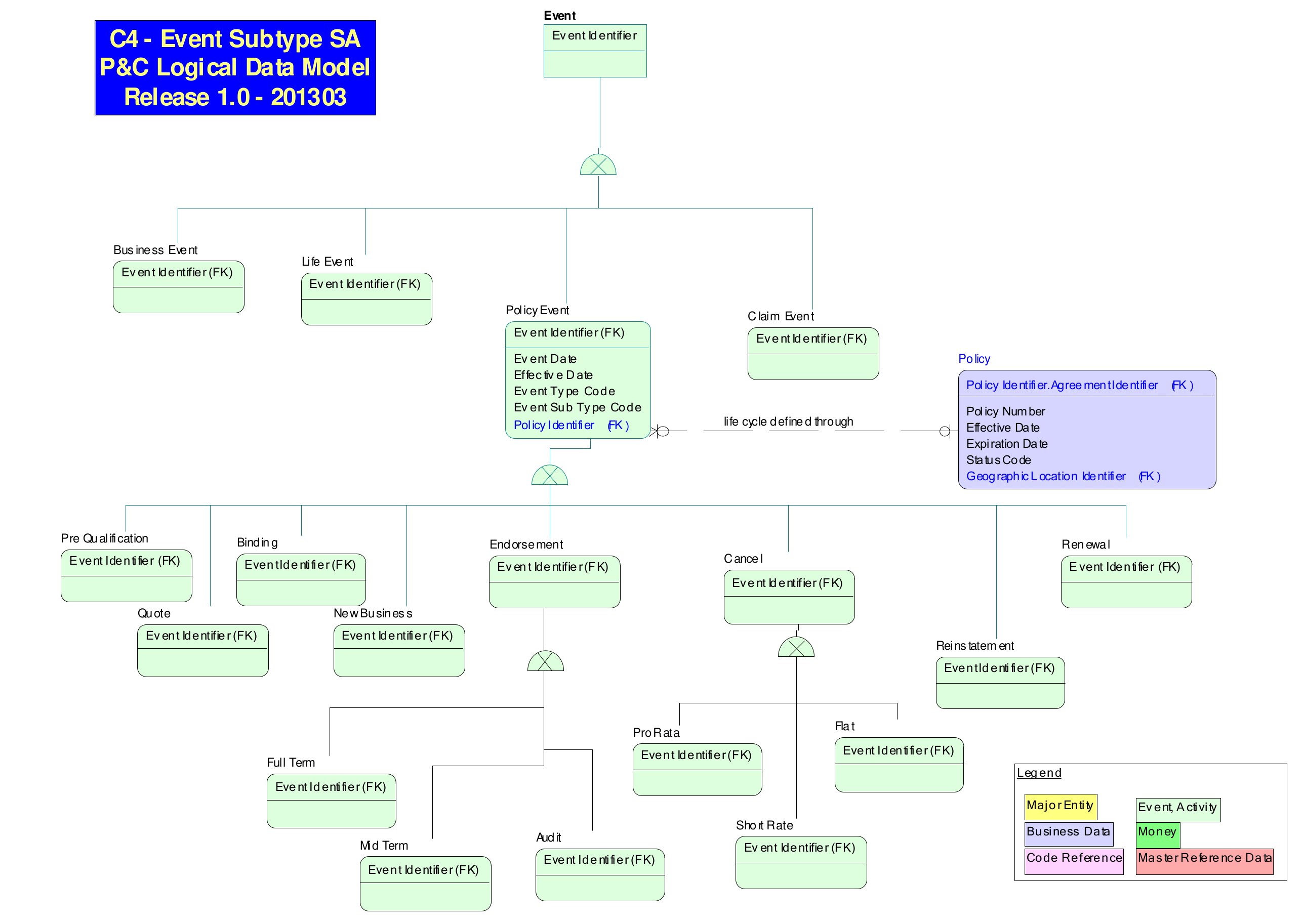
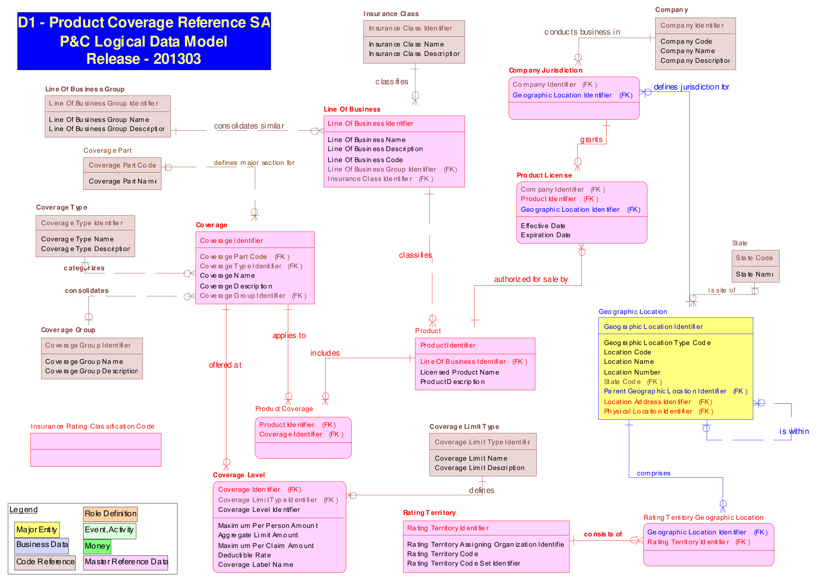
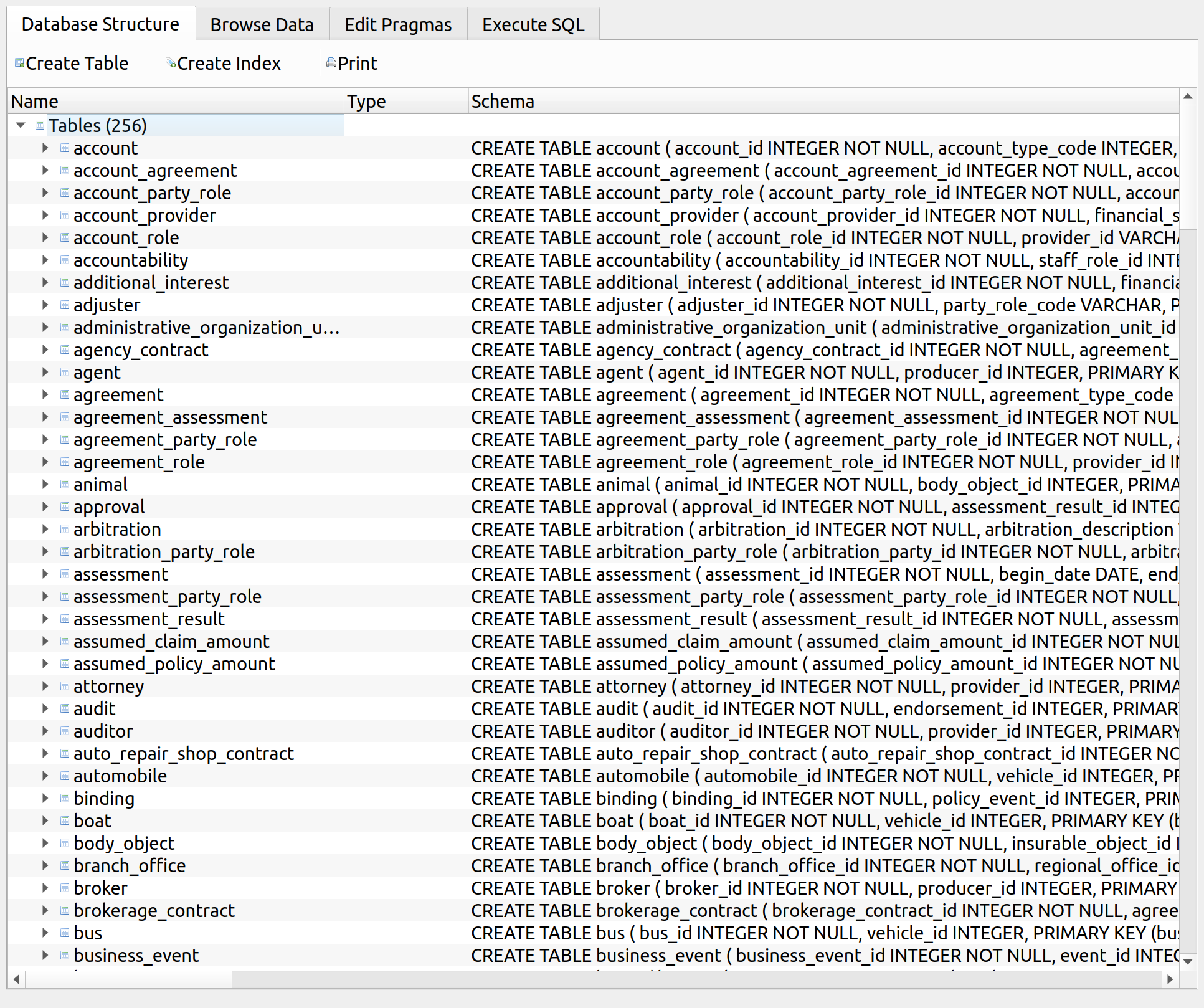
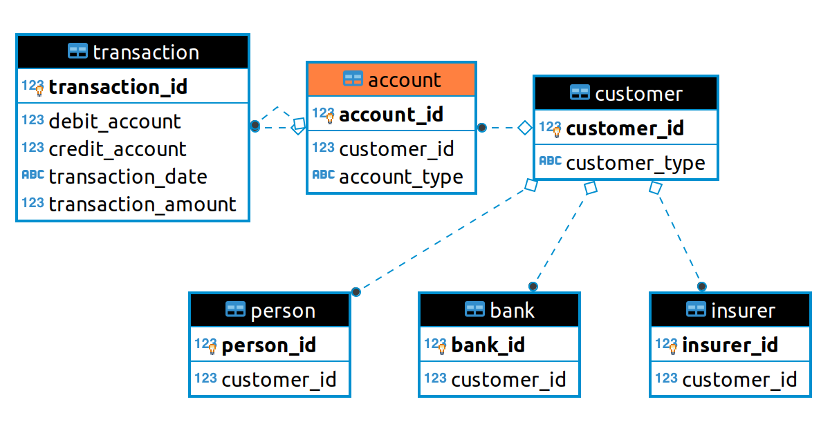
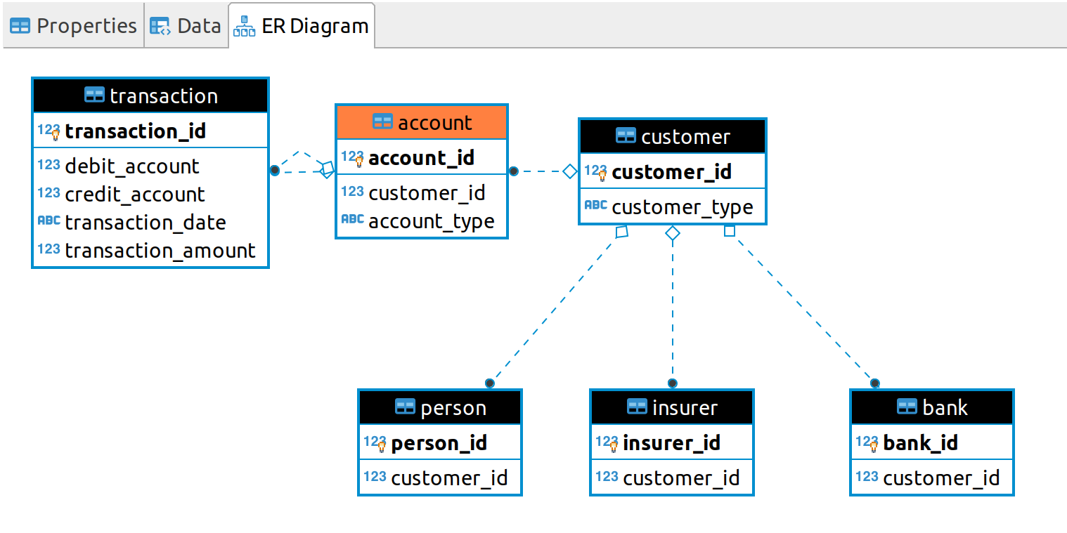
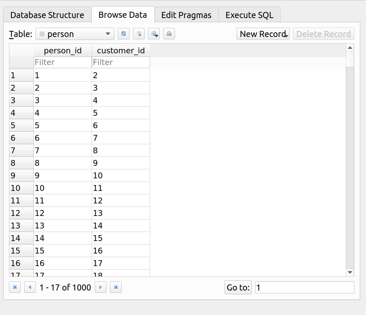
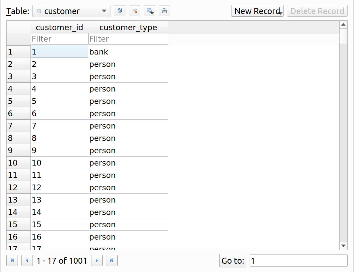
Last week, I took a break from MIES to focus on PCDM, a relational database specification for the P&C insurance industry. This week, I’m back to making progress on the consumer behavior portion of MIES, by shifting the focus from personal income to the personal endowment as the main financial constraint underlying purchasing decisions.
In short, an endowment is the consumer’s assets. When making consumption choices, people can use their income to purchase goods and services, but they can also draw from assets that they have accumulated over time, such as from savings and checking accounts, and by selling goods that they own. Furthermore, by taking the endowment into consideration, we will now be able to model situation when a person might not have a regular income, but can still make purchases using their assets (such as unemployed or retired persons who are not working).
In the context of insurance, the endowment is important because people purchase insurance to indemnify themselves against events that might damage or reduce the value of their assets. In the absence of the endowment, we would ignore an important determinant of insurance purchasing behavior. Incorporating wealth into MIES will take some time, and the textbook material I need to work on spans five chapters of Varian. Therefore, I estimate that this process will take me at least a month to do:
- Endowment
- Intertemporal Choice
- Asset Markets
- Uncertainty
- Risky Assets
These concepts will involve making some substantial changes to the utility functions as well. For now I’ll start with the endowment, which required me to modify the Budget, Slutsky, and Hicks classes of MIES.
The Endowment Class
An endowment is a bundle of goods or services that has a value based on the sum product of their prices and quantities:
![\[p_1 \omega_1 + p_2 \omega_2 = m \]](https://genedan.com/wp-content/ql-cache/quicklatex.com-b19051565e7663aa104adb787413048c_l3.png "Rendered by QuickLaTeX.com")
Where m represents income, each omega represents the quantity of each good, and each p represents the price. Rather than treat income as a flow quantity from an external source, in this interpretation of consumer choice theory we, we treat income as a stock quantity that includes the assets of of the consumer – that is, what the consumer has to spend at a certain point of time depends on the valuation of their assets.
This definition of income loosens the assumption of fixed income that I had made until now. This is because changes in asset values can now impact a person’s income. For example, if a person has a car and a house, their depreciation or appreciation changes the amount the person can sell them for on the market.
The good news is that MIES already has much of the machinery already coded up to allow us to work with endowments, so the new class definition is quite simple:
|
1 2 3 4 5 6 7 8 9 10 11 12 13 14 15 16 17 |
class Endowment: def __init__( self, good_x: Good, good_y: Good, good_x_quantity: float, good_y_quantity: float, ): self.good_x = good_x self.good_y = good_y self.good_x_quantity = good_x_quantity self.good_y_quantity = good_y_quantity @property def income(self): income = self.good_x.price * self.good_x_quantity + self.good_y.price * self.good_y_quantity return income |
An endowment takes two goods, and their quantities. Upon initialization, Python will automatically calculate the Endowment’s value by multiplying the prices of the goods by the quantities supplied. I wrote this function as a property decorator, which was introduced to fix a bug I discovered when working with the Budget class. Earlier, changing the price of a good failed to change the budget constraint of a consumer, but the property decorator will now dynamically calculate certain attributes that depend on the price, such as income in the case of an endowment.
To illustrate, we can define two goods, each with a price of 1. We then initialize an endowment with a quantity of 5 for each of these goods:
|
1 2 3 4 5 6 7 |
from econtools.budget import Endowment, Good good_1 = Good(price=1, name='good_1') good_2 = Good(price=1, name='good_2') endowment = Endowment(good_x=good_1, good_y=good_2, good_x_quantity=5, good_y_quantity=5) |
Now we can check that the income was properly calculated by calling endowment.income. Since each good has a price of 1, and there are 5 of each good, the income should be 5 x 1 + 5 x 1 = 10:
|
1 2 |
endowment.income Out[4]: 10 |
Now that we have the Endowment class defined, we need to modify the other classes that used goods, such as the Budget class. Previously, the Budget class accepted two goods, an income amount, and a name to refer to the budget. Now I would like the Budget class to an accept an endowment as an alternative to specifying each good individually. The tricky part here is that in the former case, the class needs to be able to keep income fixed when the prices of goods change, but in the latter case, the income needs to change dynamically based on the prices of the goods.
To handle this, I created an alternative constructor called from_endowment() that lets you pass an endowment to the Budget class to initialize a budget object. I also created another constructor called from_bundle() that lets you define a Budget the old way more explicitly, to make it more obvious to anyone reading the code whether the budget was initialized with an endowment or individual goods:
|
1 2 3 4 5 6 7 8 9 10 11 12 13 14 15 16 17 18 19 20 21 22 23 24 25 26 27 28 29 30 31 32 33 34 35 36 37 38 39 40 41 42 43 44 45 46 47 48 49 50 51 52 53 54 55 56 57 58 59 60 61 62 63 64 65 66 67 68 69 70 71 72 73 74 75 76 77 78 79 80 81 82 83 |
class Budget: def __init__( self, good_x, good_y, income, name=None, endowment=None ): self.good_x = good_x self.good_y = good_y self.income = income self.x_lim = self.income / (min(self.good_x.adjusted_price, self.good_x.price)) * 1.2 self.y_lim = self.income / (min(self.good_y.adjusted_price, self.good_y.price)) * 1.2 self.name = name self.endowment = endowment if endowment is not None: self.__check_endowment_consistency() @classmethod def from_bundle( cls, good_x, good_y, income, name=None ): return cls( good_x, good_y, income, name ) @classmethod def from_endowment( cls, endowment: Endowment, name=None ): good_x = endowment.good_x good_y = endowment.good_y income = endowment.income return cls( good_x, good_y, income, name, endowment ) def __check_endowment_consistency(self): # raise exception if endowment is not consistent with its components if self.endowment.good_x != self.good_x: raise Exception("Endowment good_x inconsistent with budget good_x. " "It is recommended to use the from_endowment alternative " "constructor when supplying an endowment") if self.endowment.good_y != self.good_y: raise Exception("Endowment good_y inconsistent with budget good_y. " "It is recommended to use the from_endowment alternative " "constructor when supplying an endowment") if (self.endowment.income != (self.endowment.good_x_quantity * self.good_x.price + self.endowment.good_y_quantity * self.good_y.price)) | \ (self.endowment.income != self.income): raise Exception("Endowment income inconsistent with supplied good prices. " "It is recommended to use the from_endowment alternative " "constructor when supplying an endowment") if self.endowment.good_x.price != self.good_x.price: raise Exception("Endowment good_x price inconsistent with budget good_x price. " "It is recommended to use the from_endowment alternative " "constructor when supplying an endowment") if self.endowment.good_y.price != self.good_y.price: raise Exception("Endowment good_y price inconsistent with budget good_y price. " "It is recommended to use the from_endowment alternative " "constructor when supplying an endowment") ... |
And lastly, I added some consistency checks to make sure that the endowment value equals the sum product of the prices and quantities of the goods provided. The reason why these checks are here is because a person can still use the default constructor to specify each good individually along with an endowment, just based on how the arguments are defined. While this is possible, I would discourage doing this since 1) it’s less explicit than using the alternative constructors, 2) supplying the individual goods along with the endowment is redundant, and 3) it can lead to errors being thrown.
To initialize a budget by passing an endowment, simply use the alternative constructor:
|
1 |
budget_endowment = Budget.from_endowment(endowment=endowment) |
Slutsky Decomposition
The loosening of assumptions brought about by the endowment introduces some changes to the Slutsky equation. In the examples I provided a few weeks ago, we assumed that income remained fixed when prices changed. Since changes in price now change the value of the endowment, we must now account for this change in the Slutsky equation. The derivation of this modified form can be found in Varian, so I’ll skip to the result:
![\[\frac{\Delta x_1}{\Delta p_1} = \frac{\Delta x_1^s}{\Delta p_1} + (\omega_1 - x_1)\frac{\Delta x_1^m}{\Delta m}\]](https://genedan.com/wp-content/ql-cache/quicklatex.com-e127787d64731925db6ef6b1ff0e45d9_l3.png "Rendered by QuickLaTeX.com")
The Slutsky equation can now be explained by three effects: the substitution and ordinary income effects, which are the same as before, and an endowment effect, which models how consumer choice changes when the value of the endowment changes.
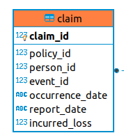
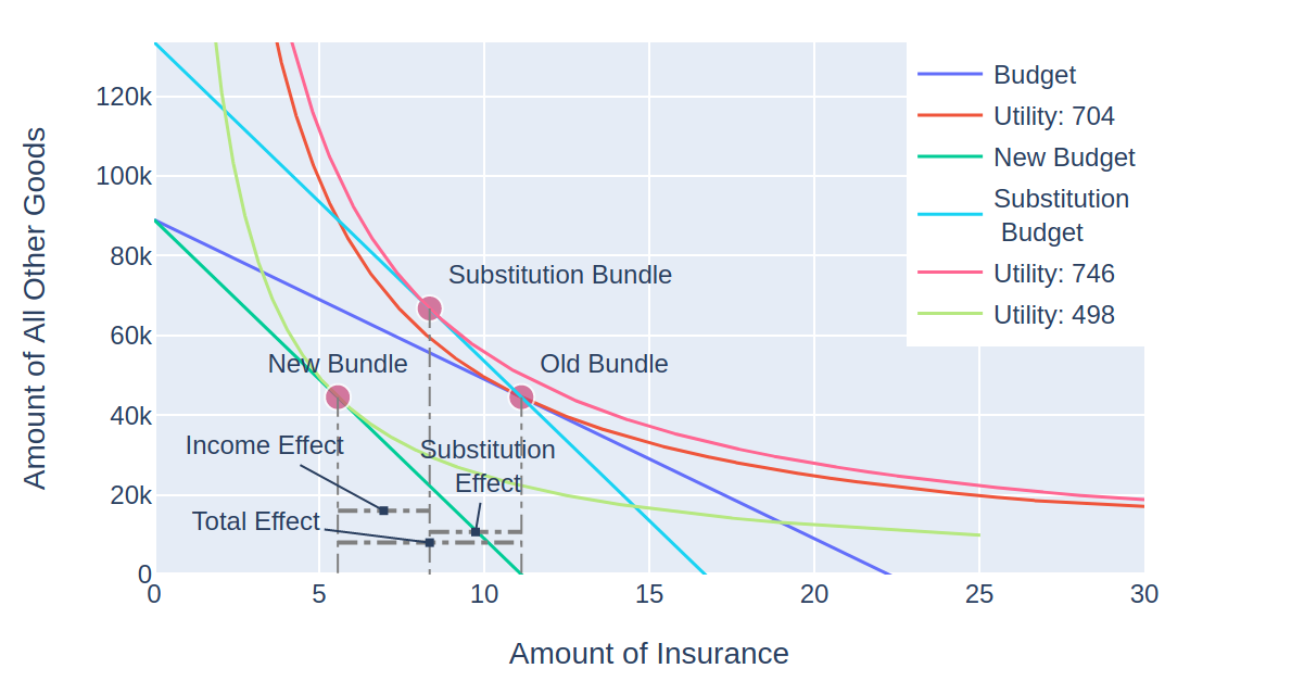
Like the Budget class, the Slutsky class has been modified to take budgets that were constructed from individual goods or an endowment. Plotting the Slutsky class is now quite bit messier, since a new budget line, bundle, and utility curve are now added to an already crowded plot.
I have not yet gotten endowments to work within the context of insurance, so the image below comes from a modified version of an example provided in Varian where a milk producer faces a $1 increase in the price of milk – his endowment increases in value, and hence income. However with the graph as cluttered as it is, it can be hard to visually isolate the effects:
It does look better with a larger plotting area if you try it with MIES, but not so much when I have to shrink the image to fit it within the margins here.
![\[\frac{\Delta x_1}{\Delta p_1} = \frac{\Delta x_1^s}{\Delta p_1} - \frac{\Delta x_1^m}{\Delta m}x_1\]](https://genedan.com/wp-content/ql-cache/quicklatex.com-267df81a1e9f4fd29a64d1fdaf119964_l3.png "Rendered by QuickLaTeX.com")
 represents the quantity of good 1 (in this case insurance),
  represents the price of insurance (that is, the premium) and
  represents the consumer’s income. The deltas are used to describe how the quantity of insurance purchased changes with premium, expressed on the left side of the identity. The first term after the equals sign represents the substitution effect, and the second term after the equals sign represents the income effect.
 ):
):![\[\Delta x_1 = \Delta x_1^s + \Delta x_1^n\]](https://genedan.com/wp-content/ql-cache/quicklatex.com-7b29a37678e0e5699894f293d45692e6_l3.png "Rendered by QuickLaTeX.com")
![\[\Delta m = x_1 \Delta p_1\]](https://genedan.com/wp-content/ql-cache/quicklatex.com-31da15f60d083e8875f089826d8cb193_l3.png "Rendered by QuickLaTeX.com")
![\[m^\prime = \frac{\bar{u}}{\left(\frac{c}{c +d}\frac{1}{p_1^\prime}\right)^c\left(\frac{d}{c+d}\frac{1}{p_2}\right)^d}\]](https://genedan.com/wp-content/ql-cache/quicklatex.com-7b6922ae6c1c86720257822287c6dbc6_l3.png "Rendered by QuickLaTeX.com")
 is the adjusted income, and
  is the new premium, and
  is the utility fixed at the original level.