• Home
  • Readings
  • Github
  • MIES
  • TmVal
  • About
Gene Dan's Blog

Category Archives: Logs

No. 79: First Post of 2013!

8 January, 2013 2:55 AM / Leave a Comment / Gene Dan

I’d like to start the new year with a few short updates:

-I ended up passing MFE back in November. I received a score of 8 (I’m assuming 9 was the highest possible score for my exam), which is one point lower than I would have liked, but nevertheless I’m happy to say that I’m finally done with the preliminary exams and halfway through with the CAS examination process. While I was waiting for my score, I also passed the CA1 module, which isn’t an ‘exam’ (even though it involves one), but one of two, month-long courses I have to take in addition to the exam requirements.

-I recently rotated into a new role at work. Instead of doing traditional reserving, I’ll be doing predictive modeling work full-time under a new supervisor. I had learned about the departmental changes after I took MFE. About a year ago, I began taking on additional responsibilities with modeling, and I’m glad to have been given the opportunity to specialize in this field. There will be a steep learning curve along the way, but I think I’ll gain valuable experience over the next couple of years.

-I didn’t manage to keep my resolution of posting 1 post per week last year. However, I managed to crank out 37 posts, which almost doubled the number of posts I had written from 2008-2011. I had steady updates until the last 3rd of the year when I stopped posting to devote time to courses MFE and CA1, but this year I’ll try my best to maintain the 1 post/week rate. I have some exciting projects that I’m currently working on, so I have a feeling I’ll easily surpass that goal.

-I installed some productivity tools in my browser to monitor the amount of time I spend on the internet. Towards the end of the year, I discovered that I sometimes wasted 6 hours in a single day due to unnecessary internet surfing on sites such as Facebook and Reddit. I also obsessively kept up with the news (ironically, in the past I had trouble keeping up with current events due to schoolwork), which oftentimes left me reading multiple articles over the same subject. I had dabbled with such browser plugins over the past couple of years, but removed them several times due to lack of discipline. This year I resolve to keep the current rules enforced for good. This year I’ve set a window from 9:00 PM to 10:00 PM devoted to social media, sports, news, and related websites (which also means I’ll have to plan my blog posts ahead of time so I can publish them within that window). At all other times during the day access will be blocked so that I can focus on doing my work, and learning the things I want to learn. I believe that strict observation of this rule will allow me to complete a lot more of my projects.

-I started studying for CAS Exam 5 this month. This gives me 4 months of solid study time for my first upper-level examination. At this point, the exams stop being math-intensive, and focus more on insurance industry practices, regulation, and law. While studying for the preliminary exams, I was so overwhelmed with math that I couldn’t focus on learning maths more relevant to my specific job (the math in the exams is related in a background sense, but as far as work goes the actual math I use is much different), along with pure math that I’ve always been wanting to learn. Although the upper examinations require more study time, I think the reduction in math required will let me spend my ‘math energy’ elsewhere.

-I’ve finished up learning the basics of SQL (as in, I’ve finished reading Learning SQL). I’m currently reading Excel & Access Integration, which I believe will give me some very useful skills with respect to data manipulation. Many actuaries know VBA, many actuaries know SQL, but there aren’t a lot of actuaries who can integrate them together effectively, so if I can acquire this ability I’ll be able to fulfill a niche role that’s lacking at many companies. I didn’t find MySQL difficult, and query writing came naturally since I had already been using MSAccess intensively 6 months before picking up the book. The only things I found difficult were correlated subqueries and the chapters on low-level database design and administration. The next thing I have on my reading list is Using R for Introductory Statistics. I actually read through the first 60 pages or so in 2011 before I stopped to study for C/4. I hope to get that finished up before March when things get really busy.

Posted in: Logs / Tagged: Actuarial Exams, exam MFE, exam mfe pass mark, exam MFE score, Learning SQL, predictive modeling, R

No. 78: Project Euler #1

30 November, 2012 3:45 AM / 1 Comment / Gene Dan

Hey everyone,

I took a few weeks off posting in order to study for Exam MFE, which I took 4 weeks ago. I’m still waiting for the result, so in the meantime I’ve decided to knock out the CAS modules and finish up my SQL course before I have to start studying hard again. Anyway, I’ve finally gotten around to attempting the Project Euler problems that my friends, along with other actuaries, recommended to me as a good way to improve my programming skills.

Basically, Project Euler is a website that hosts mathematical problems that anyone can attempt to solve with whatever method they wish. Most of the problems are simply stated and can be understood by most people who have taken a basic course in number theory. However, they are often very computationally intensive if attempted directly so most people try to solve them by writing computer programs. Oftentimes students will use the site in an iterative fashion to practice their programming skills when picking up a new language. For example, one of my colleagues who has solved 80 problems first used the site to learn VBA, and then did the same problems again in R, and then again in C++.

For my first attempt, I decided to use VBA because I already know most of the basic syntax. Before starting, I decided that I would not seek any outside help or lookup any solutions when trying to solve these problems, because I want to work these out on my own. So please don’t give me any tips! (although I do appreciate any advice for any of my other projects).

The first problem is stated as follows:

If we list all the natural numbers below 10 that are multiples of 3 or 5, we get 3, 5, 6 and 9. The sum of these multiples is 23.

Find the sum of all the multiples of 3 or 5 below 1000.

Solution:

[code language=”vb”]
Sub euler1()

Dim x As Long ‘natural number to be tested
Dim y As Long ‘current sum of the multiples of 5 or 3

y = 0
For x = 1 To 999
If x Mod 3 = 0 Or x Mod 5 = 0 Then
y = y + x
End If
Next x

Debug.Print y

End Sub
[/code]

The final output is 233168. As you can see, the problem is quite easy to understand (and this one was very easy to solve as well) for anyone who passed grade school math. You can probably solve it by sitting at your desk and adding every multiple of 3 or 5 below 1000 by hand, but that would be extremely boring and you probably have better things to do. That’s why you write a program to solve the problem. The solution I wrote above is a simple brute force method (I tested every natural number below 1000 to see if it was evenly divided by 3 or 5) that took less than a second for my computer to solve. The key to understanding the solution is the mod operator, which returns the remainder in a division operation (for example 5 mod 3 equals 2). The statement “If x Mod 3 = 0 Or x Mod 5 = 0” tells the computer to execute the subsequent line, or to add x to the cumulative sum if either x mod 3 or x mod 5 equals 0, in other words, if the remainder after dividing x by 3 or 5 is 0.

So far I’ve solved 17 of the problems, mostly through brute force although I was able to solve one of them by hand. However, as the problems get progressively harder and more computationally intensive, brute force methods become less feasible and more creative thought is required. For example, problem 12 took my computer at least an hour to solve (I’m not sure how long it actually took because I left it on after I went to sleep). This means my solution wasn’t efficient, and that I ought to give it another shot (reduce the amount of iterative code, perhaps).
Posted in: Logs, Mathematics / Tagged: project euler, project euler #1, project euler vba, VBA

No. 77: Stochastic Calculus on a Friday Night

13 October, 2012 2:21 AM / Leave a Comment / Gene Dan

\[\int^a_b \mathrm{d}Z(t) = \lim_{n \to \infty} \sum^n_{i=1}\left(Z\left(\frac{ia}{n}\right)-Z\left(\frac{(i-1)a}{n}\right)\right) \]
Hey everyone,

I’m struggling to absorb all the material necessary to pass MFE, but if I can just plow through the 3 remaining chapters I think I’ll be OK. I keep telling myself not to freak out because everyone else says that the last quarter of MFE is notoriously difficult. You’re not expected to master the theoretical details of Brownian motion or Itô processes but you are expected to be able to understand the basics and be able to manipulate mathematical expressions to make meaningful calculations – such as pricing bonds and options – but even that can be intimidating, especially to those (like me) who haven’t taken a course on differential equations.

The figure above represents a stochastic integral – this is kind of like the type of integral you learned in elementary calculus except in this case the function Z(t) is not a fixed function – it is a function that returns a random value from a normal distribution whose parameters vary with respect to time. This particular integral calculates the movement of a stock price from time b to time a. Another thing we might want to model is the total variation of the process – which is the arc length of the stock price trajectory (we use the absolute value because we want down-moves, which are negative, to add to the arc length) :
\[ \lim_{n to \infty}\sum^n_{i=1}\left|X\left(\frac{iT}{n}\right)-X\left(\frac{(i-1)T}{n}\right)\right| \]
An interesting note is that as n approaches infinity, the probability the trajectory crosses its starting point an infinite number of times equals 1 (I have a hard time imagining this).

The image below is a visual representation of Brownian motion with different shades of blue representing a different number of steps. Note that this wouldn’t be appropriate for stock prices because ideally, we would want the trajectory to only traverse positive time and value:

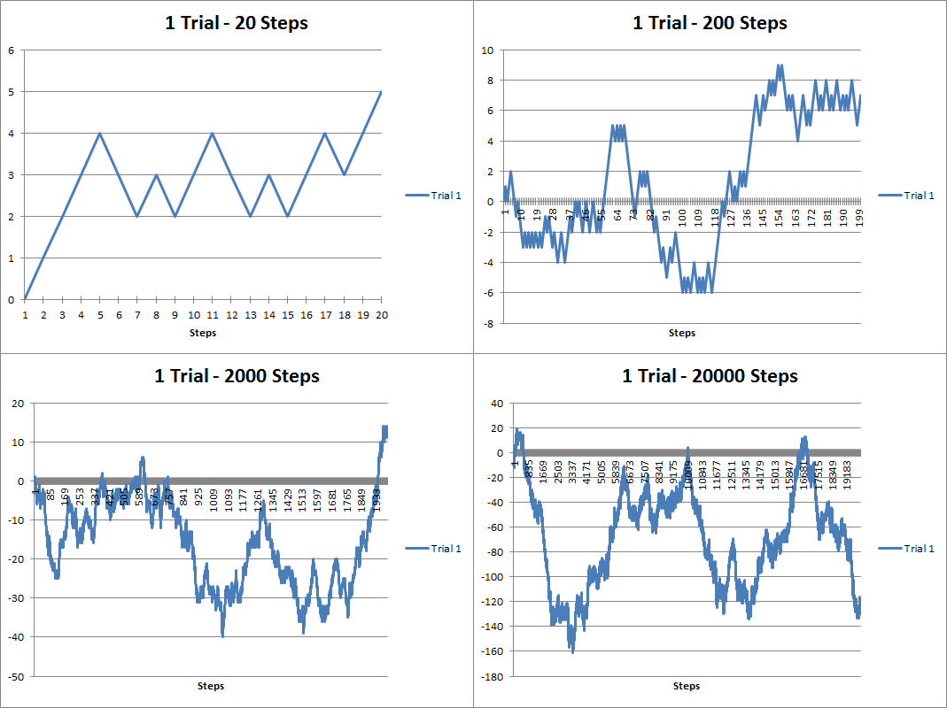
Anyway, over a year ago I dabbled with some discrete stochastic processes using VBA. Here are some random walks I generated:

The above figure are random walks generated using 20, 200, 2000 and 20000 steps. You can see that it looks kind of like a stock chart except the values can be negative. As the number of steps increases, the trajectory looks more like a curve. Brownian motion is when the number of steps becomes infinitely large and the time between steps infinitely small. Below you’ll see that I’ve overlapped several trials below. As the number of trials increases, you can see that the results take up more and more of the possible trajectory space:

About a year and a half ago I had created a youtube video showing how you can animate the random walks in VBA:

Here’s part of the source code I used to generate the walks:

[code language=”vb” wraplines=”TRUE” collapse=”TRUE”]

Sub randwalk()

Dim x As Double
Dim y As Long, z As Double, m As Integer, n As Integer, s As Integer
Dim randarray() As Double
Dim ymax As Integer
Dim ChtObj As ChartObject
Dim Steps As Double, Trials As Double
Dim stup As Double, stdown As Double
Dim pstup As Double, pstown As Double
Dim frate As Double

starttime = Timer

Application.ScreenUpdating = False

For Each ChtObj In Worksheets(“Graph”).ChartObjects
ChtObj.Delete
Next ChtObj

Worksheets(“Data”).UsedRange.Clear

Steps = Range(“STEPS”).Value
Trials = Range(“TRIALS”).Value
stup = Range(“STUP”).Value
stdown = Range(“STDOWN”).Value
pstup = Range(“PSTUP”).Value
frate = Range(“FRATE”).Value

ReDim randarray(0 To Steps) As Double

For m = 0 To Trials – 1
z = Range(“STARTVAL”).Value
randarray(0) = Range(“STARTVAL”).Value
For y = 1 To Steps
x = Rnd()
If x >= (1 – pstup) Then x = stup Else x = -1 * stdown
If Range(“FTYPE”).Value = “Arithmetic” Then
z = z + x
Else
z = z * (1 + x)
End If
randarray(y) = z
Next y
Worksheets(“Data”).Range(“A1”).Offset(0, m).Value = “Trial ” & m + 1
Worksheets(“Data”).Range(“A2:A” & Steps + 1).Offset(0, m) = WorksheetFunction.Transpose(randarray)
Next m

If Range(“COMP”).Value = “Yes” Then
For n = 1 To Steps
randarray(n) = randarray(n – 1) * (1 + frate)
Next n

Worksheets(“Data”).Range(“A1:A” & Steps + 1).Offset(0, Trials) = WorksheetFunction.Transpose(randarray)
End If

Dim MyChart As Chart
Dim DataRange As Range
Set DataRange = Worksheets(“Data”).UsedRange
Set MyChart = Worksheets(“Graph”).Shapes.AddChart.Chart
MyChart.SetSourceData Source:=DataRange
MyChart.ChartType = xlLine

With Worksheets(“Graph”).ChartObjects(1)
.Left = 1
.Top = 1
.Width = 400
.Height = 300
.Chart.HasTitle = True
If Trials = 1 Then
.Chart.ChartTitle.Text = Trials & ” Trial – ” & Range(“FTYPE”).Value & ” Progression”
Else
.Chart.ChartTitle.Text = Trials & ” Trials – ” & Range(“FTYPE”).Value & ” Progression”
End If
.Chart.PlotBy = xlColumns

End With

With MyChart.Axes(xlCategory)
.MajorTickMark = xlTickMarkCross
.AxisBetweenCategories = False
.HasTitle = True
.AxisTitle.Text = “Steps”
End With

For s = 1 To Trials
MyChart.SeriesCollection(s).Name = “Trial ” & s
Next s

If Range(“COMP”).Value = “Yes” Then
MyChart.SeriesCollection(Trials + 1).Name = “Fixed Growth”
MyChart.SeriesCollection(Trials + 1).Interior.Color = “black”
End If

Range(“MAXVAL”).Value = WorksheetFunction.Max(Worksheets(“Data”).UsedRange)
Range(“MINVAL”).Value = WorksheetFunction.Min(Worksheets(“Data”).UsedRange)
Range(“EXECTIME”).Value = Format(Timer – starttime, “00.000”)

Application.ScreenUpdating = True

End Sub
[/code]

Posted in: Logs / Tagged: Actuarial Exams, brownian motion, exam MFE, random walks, stochastic calculus, stochastic processes, VBA

No. 76: Exploring Financial Data with Quantmod

6 October, 2012 1:36 AM / 1 Comment / Gene Dan

Hey everyone,

Things have been extremely busy lately – I feel like the quality of my posts will suffer but I’ll try to put anything I find interesting here. I’m currently studying for my fifth actuarial exam – 3F/MFE – which covers models for financial economics. The exam covers the latter half of McDonald’s Derivatives Markets, which is a graduate textbook covering the basics of financial derivatives – such as forwards and options, and introduces the reader to elementary stochastic processes like random walks and Brownian Motion used to theoretically price these derivatives.

Anyway, some snooping around on the internet for open-source financial software led me to some quantitative finance packages in R – namely Quantmod, which I’ll be discussing here. Unfortunately it seems that (correct me if I’m wrong) the Quantmod project has been abandoned for some time, but its ease of use was my reason to showcase it here. It looks like other packages such as Quantlib have more active involvement – but I currently lack the technical skills/financial knowledge  to work with that, but I may revisit it later.

The example above may be a familiar image to some of you – it is a chart depicting the CBOE VIX (volatility index), which measures the implied volatility of S&P 500 index options – in other words – it is an estimate of the short-term volatility of the stock market. Notice that 2008 saw high volatility – this makes sense because the stock market plunged that year. This actually isn’t the highest value seen in the index – to my knowledge that occured on Black Monday in 1987 when the DJIA lost a quarter of its value in less than a day. The above chart was generated using Quantmod with the following code:

[sourcecode language=”r”]
library("quantmod")
getSymbols("^VIX",src="yahoo")
barChart(VIX)
[/sourcecode]

Well, that was simple. Quantmod has a function called getSymbols() that extracts the desired data. The two arguments above (there are more arguments than that – I chose to use the defaults for the rest), specify the ticker symbol to extract (^VIX) and the source of the financial data (yahoo.com). The next function, barchart, plots the data.

1
2
3
4
5
6
7
8
9
10
11
12
13
<span style="color:#0000ff;">&gt;str(VIX)</span>
An ‘xts’ object from 2007-01-03 to 2012-10-05 containing:
  Data: num [1:1453, 1:6] 12.2 12.4 11.8 12.5 11.9 ...
- attr(*, "dimnames")=List of 2
  ..$ : NULL
  ..$ : chr [1:6] "VIX.Open" "VIX.High" "VIX.Low" "VIX.Close" ...
  Indexed by objects of class: [Date] TZ:
  xts Attributes:  
List of 4
$ tclass : chr [1:2] "POSIXct" "POSIXt"
$ tzone  : chr ""
$ src    : chr "yahoo"
$ updated: POSIXct[1:1], format: "2012-10-05 20:02:43"

The output above tells us that the variable VIX is a time-series object (xts) from January 1st, 2003 to today. The following is the output of the first 10 rows of daily data:

1
2
3
4
5
6
7
8
9
10
11
12
13
&gt;VIX[1:10]
<span style="color:#000000;">           VIX.Open VIX.High VIX.Low VIX.Close VIX.Volume VIX.Adjusted
2007-01-03    12.16    12.75   11.53     12.04          0        12.04
2007-01-04    12.40    12.42   11.28     11.51          0        11.51
2007-01-05    11.84    12.25   11.68     12.14          0        12.14
2007-01-08    12.48    12.83   11.78     12.00          0        12.00
2007-01-09    11.86    12.47   11.69     11.91          0        11.91
2007-01-10    12.34    12.50   11.43     11.47          0        11.47
2007-01-11    11.42    11.48   10.50     10.87          0        10.87
2007-01-12    10.93    10.93   10.14     10.15          0        10.15
2007-01-16    10.64    10.89   10.40     10.74          0        10.74
2007-01-17    10.90    10.90   10.35     10.59          0        10.59
</span>

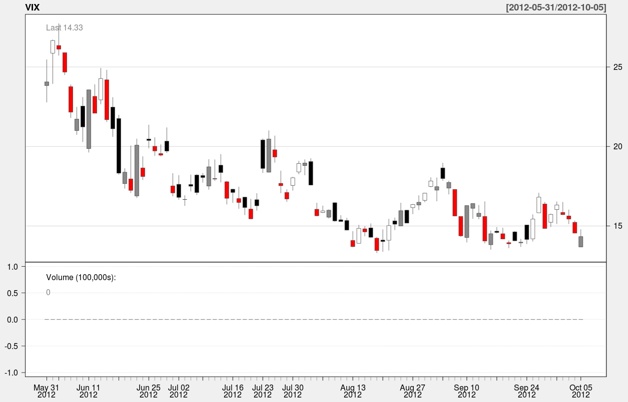
Here’s an example of a candle chart covering the last 90 days of the index:

A candle chart allows you to visualize the daily spread in addition to the trend over a longer period of time. In the above chart, the colored rectangles are bounded by the open/close values of the day, and the endpoints of the vertical line segments represent the hi/low values of the day.

The function used to generate this chart is:

[sourcecode language=”r”]
candleChart(VIX,multi.col=TRUE,theme="white",subset="last 90 days")
[/sourcecode]

The argument “subset” specifies the slice of time to be plotted in the chart. It’s nice because it accepts natural language – all I had to do was type in “last 90 days” to specify the time interval. Anyway that’s it for now – In the meantime I’ll be spending up to 4-5 hours a day preparing for my test at the beginning of next month.

Posted in: Logs, Mathematics

No. 75: A Training Update

11 September, 2012 1:30 AM / 1 Comment / Gene Dan

Hey everyone,

I feel like my training has progressed well over the last couple of months. Two weeks ago, I wrote that I would try to increase the time at which I could maintain 160-165 bpm to 60 minutes (2 x 30 minute intervals). I managed to complete this goal last Thursday without too much difficulty, though I was getting tired during the last 10 minutes of the second interval:

You can see that there were a couple of blips where I lost focus and my HR dropped below 160, but in the end, the intervals averaged out to 163 bpm and 164 bpm, and I’m satisfied with the way things turned out. This week is a transition week for me, so I’ll still be riding, but the workouts will be unstructured and “fun” to allow me to rest my legs and clear my mind before the next phase of training. The week after that, I plan to conduct a lactate threshold (the heart rate at which the activity becomes anaerobic) test, which involves doing a 30 minute TT, with the average HR of the last 20 minutes being the approximation of LT. I don’t have any big expectations for this test, but I think it will be at least 164 bpm because I know I can do that given the picture above. The first of the two intervals I did was pretty easy, and not the lung-busting effort that you’d produce during a TT. However, I haven’t done a time trial since Fayetteville, so I might not be able to get my HR that high, but I think 168 bpm would be a reasonable expectation or even maybe 170 bpm if I can get it that high.

One of the important things about LT is that cycling involves several different types of endurance: aerobic endurance, anaerobic endurance, and muscular endurance (there might be more to the list). Throughout the offseason, I’ll need to isolate these different types of endurance and create workouts to develop each one. LT is the point at which physical activity becomes anaerobic and lactic acid begins accumulating in the muscles. At this point, the body can only hold so much lactic acid before the muscles fail – and it’s crucial in bicycle racing to out-endure your opponents at critical moments during a race, such as in the final moments of a breakaway. I noticed this year that I had trouble staying with the pack during hard efforts, and this is one of the things I would like to work on before returning to racing. Therefore, in order to tailor workouts to fit my goals, I’ll need to know my LT in order to separate workouts (or parts of workouts) into aerobic/anaerobic segments.

I don’t have any plans to do anaerobic exercises yet, because it’s important to build a good amount of basic aerobic endurance during the offseason, so you’ll have enough endurance to work on high-intensity anaerobic workouts later on. Last year I didn’t ride much in the winter, and I think one of the reasons I ran into overtraining problems in the Spring was that I hadn’t built up enough endurance in the offseason. Anyway, for the next month my goal is to increase the amount of time I can ride non-stop at 160+ bpm (or whatever turns out to be right under LT). I’ll keep the total amount of time above 160+ bpm, but I’ll gradually shift the distribution of time of the 2 intervals more towards the 2nd interval. For the next 4 weeks (2 interval workouts per week):

LT Test: 1 x 30 min
1 x 20 min and 1 x 20 min

1 x 20 min and 1 x 25 min
1 x 25 min and 1 x 25 min

1 x 25 min and 1 x 30 min
1 x 30 min and 1 x 30 min

1 x 25 min and 1 x 35 min
1 x 20 min and 1 x 40 min

(Transition week + 2nd LT Test)

I would eventually like to be able to ride nonstop right below my LT for an hour. I think realistically that will be possible at the end of November. I’m planning to do long weeks for base training in November and December (10-11 hours/week), which aren’t long by competitive standards, but they’re longer than what I did last year and what I believe to be a reasonable goal for the offseason.

Weights

Weight training has continued as usual:

Squat: 5×5 195 lb
Deadlift: 1×5 185 lb
Bench: 5×5 130 lb
Overhead press: 5×5 80 lb
Weighted Dips: 5×5 40 lb
Barbell Row: 5×5 125 lb
Weighted Pullups: 5×5 2.5 lb
Power Clean 3×5 90 lb

I’m planning to do most of my gains this Winter and next Summer when racing is light. I realized this year that it’s really hard to make gains during Spring when all the races are going on.

Posted in: Cycling, Logs

Post Navigation

« Previous 1 … 4 5 6 7 8 … 19 Next »

Archives

  • September 2023
  • February 2023
  • January 2023
  • October 2022
  • March 2022
  • February 2022
  • December 2021
  • July 2020
  • June 2020
  • May 2020
  • May 2019
  • April 2019
  • November 2018
  • September 2018
  • August 2018
  • December 2017
  • July 2017
  • March 2017
  • November 2016
  • December 2014
  • November 2014
  • October 2014
  • August 2014
  • July 2014
  • June 2014
  • February 2014
  • December 2013
  • October 2013
  • August 2013
  • July 2013
  • June 2013
  • March 2013
  • January 2013
  • November 2012
  • October 2012
  • September 2012
  • August 2012
  • July 2012
  • June 2012
  • May 2012
  • April 2012
  • March 2012
  • February 2012
  • January 2012
  • December 2011
  • September 2011
  • August 2011
  • July 2011
  • June 2011
  • January 2011
  • December 2010
  • October 2010
  • September 2010
  • August 2010
  • June 2010
  • May 2010
  • April 2010
  • March 2010
  • September 2009
  • August 2009
  • May 2009
  • December 2008

Categories

  • Actuarial
  • Cycling
  • Logs
  • Mathematics
  • MIES
  • Music
  • Uncategorized

Links

Cyclingnews
Jason Lee
Knitted Together
Megan Turley
Shama Cycles
Shama Cycles Blog
South Central Collegiate Cycling Conference
Texas Bicycle Racing Association
Texbiker.net
Tiffany Chan
USA Cycling
VeloNews

Texas Cycling

Cameron Lindsay
Jacob Dodson
Ken Day
Texas Cycling
Texas Cycling Blog
Whitney Schultz
© Copyright 2025 - Gene Dan's Blog
Infinity Theme by DesignCoral / WordPress