• Home
  • Readings
  • Github
  • MIES
  • TmVal
  • About
Gene Dan's Blog

Category Archives: Logs

No. 66: CPU Stress Testing with GIMPS

17 July, 2012 1:29 AM / Leave a Comment / Gene Dan

Hey everyone,

Last week I wrote about liquid cooling and overclocking my Linux server. I spent that Sunday mostly fiddling around with the CPU multiplier and voltage settings, but I didn’t subject the machine to any lengthy stress testing because I mainly wanted to see how high I could safely overclock the core. My friend Daniel told me that if I wanted to truly test the stability of a particular overclock setting, I’d have to test the computer over the course of several hours to make sure the programs ran correctly and that no wild temperature fluctuations took place. Furthermore, I’d have to run two separate batteries of tests – (one with the AC on and one without) to make sure that the machine wouldn’t overheat without air conditioning.

Unfortunately, I couldn’t complete the entire experiment because it rained almost every day last week (and will continue to rain each day this week), which meant that the temperatures wouldn’t be hot enough outside (hence, inside) to test the machine under summer conditions. However, I still had the opportunity to see how the computer would operate in cool conditions, which I had originally intended to do as a control. Thus, I decided to test the CPU using GIMPS at 5 clock settings: 3200 MHz, 3360 MHz, 3519 MHz, 3680 MHz, and 3840 MHz – with 3200 MHz as the stock setting.

Stress testing at 3840 MHz

The test was simple. I’d first use the terminal to dump the motherboard’s temperature readings into a text file, run GIMPS over the course of a workday (at least 9 hours), and then import the results of the test into an Excel spreadsheet to compare the results. I was able to find some code on how to make the text file by searching ubuntuforums.org, from which I used the following loop to log the temperatures each minute over the course of each test:

while true; do sensors >> log.txt; sleep 60; done

Which logged the following output each minute into a text file:

w83627dhg-isa-0290
Adapter: ISA adapter
Vcore: +1.04 V (min = +0.00 V, max = +1.74 V)
in1: +0.00 V (min = +0.06 V, max = +1.99 V) ALARM
AVCC: +3.28 V (min = +2.98 V, max = +3.63 V)
+3.3V: +3.28 V (min = +2.98 V, max = +3.63 V)
in4: +1.84 V (min = +0.43 V, max = +1.28 V) ALARM
in5: +1.70 V (min = +0.66 V, max = +0.78 V) ALARM
in6: +1.64 V (min = +1.63 V, max = +1.86 V)
3VSB: +3.49 V (min = +2.98 V, max = +3.63 V)
Vbat: +3.44 V (min = +2.70 V, max = +3.30 V) ALARM
fan1: 0 RPM (min = 2636 RPM, div = 128) ALARM
fan2: 2163 RPM (min = 715 RPM, div = 8)
fan3: 0 RPM (min = 1757 RPM, div = 128) ALARM
fan5: 0 RPM (min = 2636 RPM, div = 128) ALARM
temp1: +27.0°C (high = +0.0°C, hyst = +100.0°C) sensor = thermistor
temp2: +27.0°C (high = +80.0°C, hyst = +75.0°C) sensor = thermistor
temp3: +32.0°C (high = +80.0°C, hyst = +75.0°C) sensor = thermistor

k10temp-pci-00c3
Adapter: PCI adapter
temp1: +27.5°C (high = +70.0°C)

radeon-pci-0200
Adapter: PCI adapter
temp1: +55.5°C

You can see that the above output is quite cryptic – and it took me a while searching the forums until I found out that the CPU reading was denoted by “k10temp-pci-00c3.” Because the loop recorded these temperatures every minute, I was able to use the fact that each temperature reading repeated every 27 lines to write a loop in VBA and extract these readings into an Excel spreadsheet:

Option Explicit

Sub import_temperatures()
Dim r As Long, m As Long
Dim temperature As String

Range("A2:E1000000").Clear

Open "C:UsersGeneDesktop3840.txt" For Input As #1

r = 1
m = 0
Do Until EOF(1)
Line Input #1, temperature
If r = 16 Or ((r - 16) Mod 27 = 0) Then
Range("A2").Offset(m, 0).Value = Right(Left(Trim(temperature), 19), 4)
ElseIf r = 17 Or (r - 17) Mod 27 = 0 Then
Range("B2").Offset(m, 0).Value = Right(Left(Trim(temperature), 19), 4)
ElseIf r = 18 Or (r - 18) Mod 27 = 0 Then
Range("C2").Offset(m, 0).Value = Right(Left(Trim(temperature), 19), 4)
ElseIf r = 22 Or (r - 22) Mod 27 = 0 Then
Range("D2").Offset(m, 0).Value = Right(Left(Trim(temperature), 19), 4)
ElseIf r = 26 Or (r - 26) Mod 27 = 0 Then
Range("E2").Offset(m, 0).Value = Right(Left(Trim(temperature), 19), 4)
m = m + 1
End If
r = r + 1
Loop

Close #1

End Sub

The test took 5 days to complete, so I had to be patient. Here are the results:

Stress Testing Results at 100% Load

You can see that the results are very impressive. At stock settings, the CPU temperature hovered at around 45 degrees Celsius at 100% effort. This means that I can leave the computer on all day and even the most intensive task won’t push the temperature past 50 degrees (or not even past 47 degrees). Even at 3840 MHz, the temperature stayed at around 55 degrees Celsius over the course of 9 hours. I did however, have to increase the voltage for clock speeds of 3519 MHz and above, so I’m not sure if the temperature increases beyond that speed were due to voltage increases, multiplier increases, or a combination of both. Moreover, I’m not sure if the increased clock speeds made GIMPS run any faster, since the per-iteration time seems to depend on which exponent you are testing (I’m sure there’s a way, though).  Nevertheless, I’m very satisfied with the results and the ability of the liquid cooling system to keep temperatures stable while I’m away from home.

Posted in: Logs / Tagged: corsair h80, cpu benchmarking, GIMPS, liquid cooling, mprime, overclocking, overclocking AMD phenom II, prime 95

No. 65: Liquid Cooling & Overclocking

10 July, 2012 1:59 AM / 1 Comment / Gene Dan

Hey everyone,

A while back I wrote about a Linux server I set up in order to do statistical work remotely from other computers. So far, I haven’t done much with it other than learn R and LaTeX, but recently I’ve discovered that it would be a great tool to document some of the algorithms I’ve developed through my modeling projects at work in the event that I would ever need to use them again (highly likely). Back in January, I wrote that I was concerned about the CPU getting too hot since I left it on at home while I was away at work. Since I leave the AC off when I’m gone, the air going into the machine would be hotter and would hinder the cooling ability of the server’s fans.

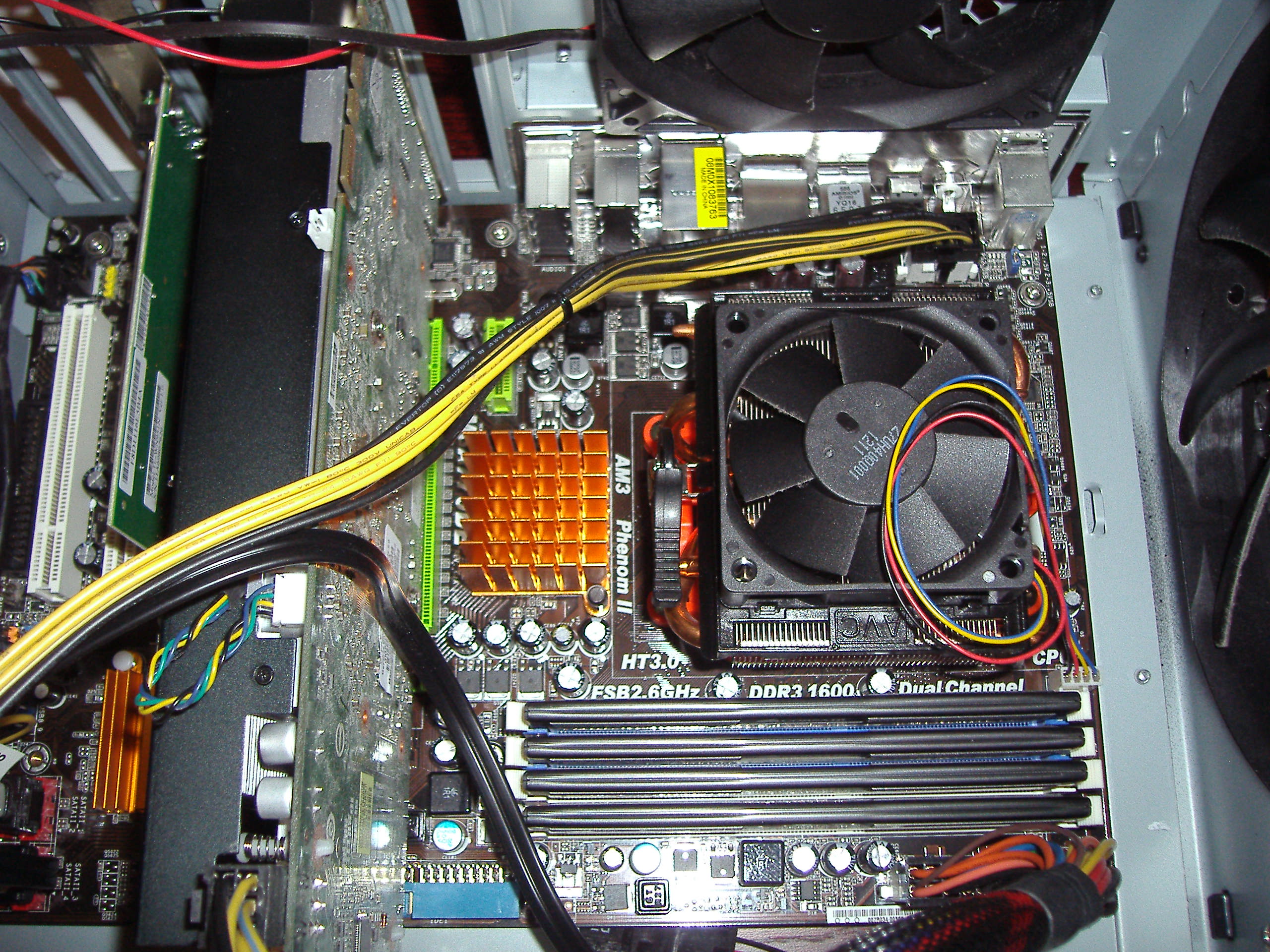
Original setup with stock AMD fan + heatsink

I could leave the AC on, but that wouldn’t be environmentally friendly, so I’ve been looking for other solutions to keep my processor cool. One of the options I decided to try was liquid cooling – which I heard was more energy efficient and better at cooling than traditional air cooling found on stock computers. Moreover, I had seen some really creative setups on overclockers.net – which encouraged me to try it myself. To get started, I purchased a basic all-in-one cooler from Corsair. This setup isn’t as sophisticated as any of the custom builds you’d see at overclockers, but it was inexpensive and I thought it would give me a basic grasp on the concept of liquid cooling.

The installation was pretty easy – all I had to do was remove the old heatsink and screw in pump/waterblock into the CPU socket. Then, I attached the 2 x 120 mm fans along with the radiator to the back of the case:

New setup with Corsair H80 system installed

However, one of the problems with these no-fuss all-in-one systems is that you can’t modify the hose length, which might make the system difficult or impossible to install if your case is too large or too small. As you can see, I got lucky – the two fans along with the radiator barely fit inside my mid-tower Antec 900 case. If it were any smaller the pump would have gotten in the way and I would have had to remove the interior fan to make it fit. Nevertheless, I’m really satisfied with the product – as soon as I booted up the machine I was impressed by how quietly it ran.

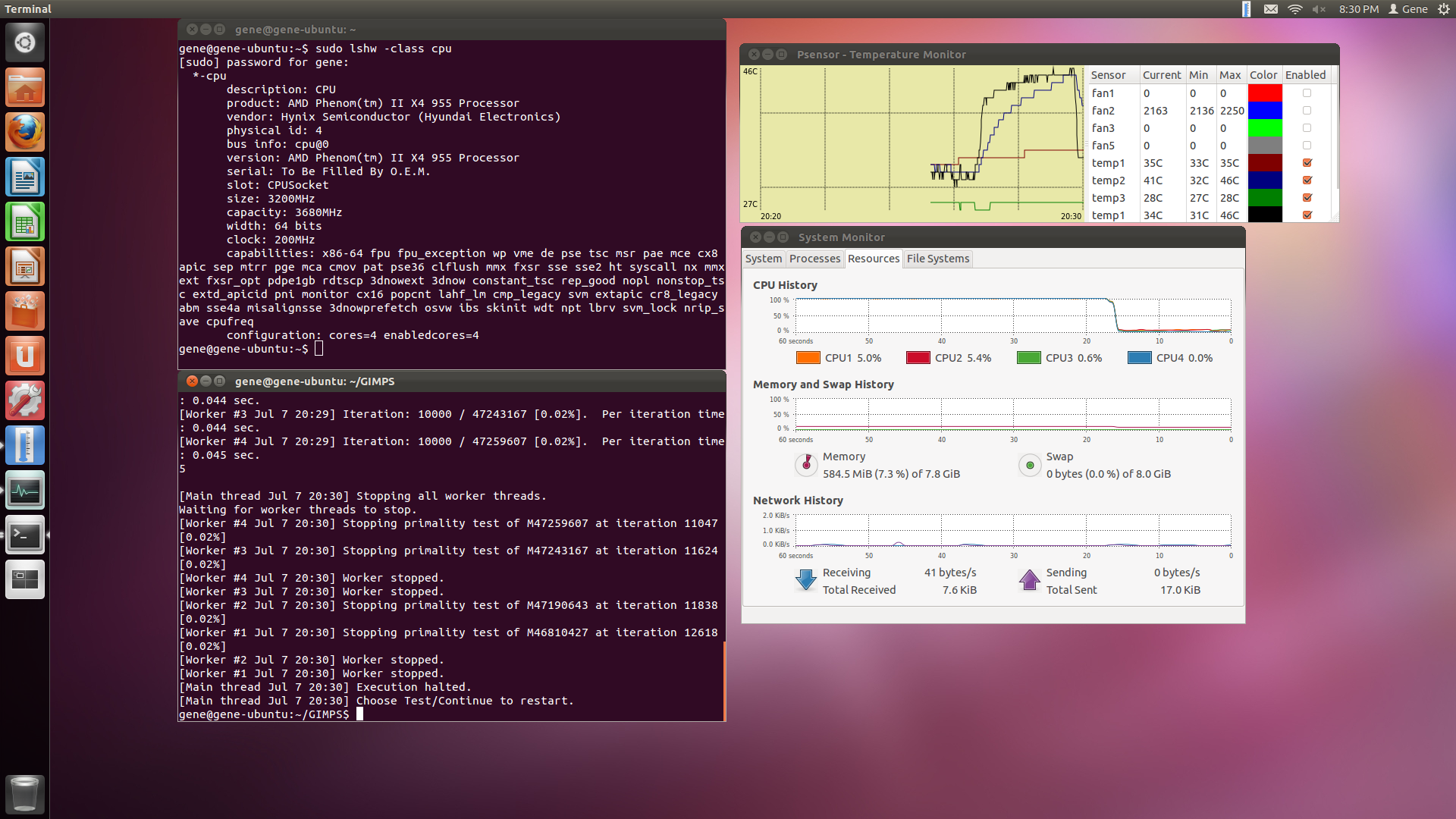
Naturally, I decided to overclock the processor to test the effectiveness of the new cooling system. I increased the clock speed of the CPU (AMD Phenom II) from 3200 MHz to 3680 MHz and ran all 4 cores at 100% capacity to see how high temperatures would get. Here are the results below:

Overclocking at 3680 MHz

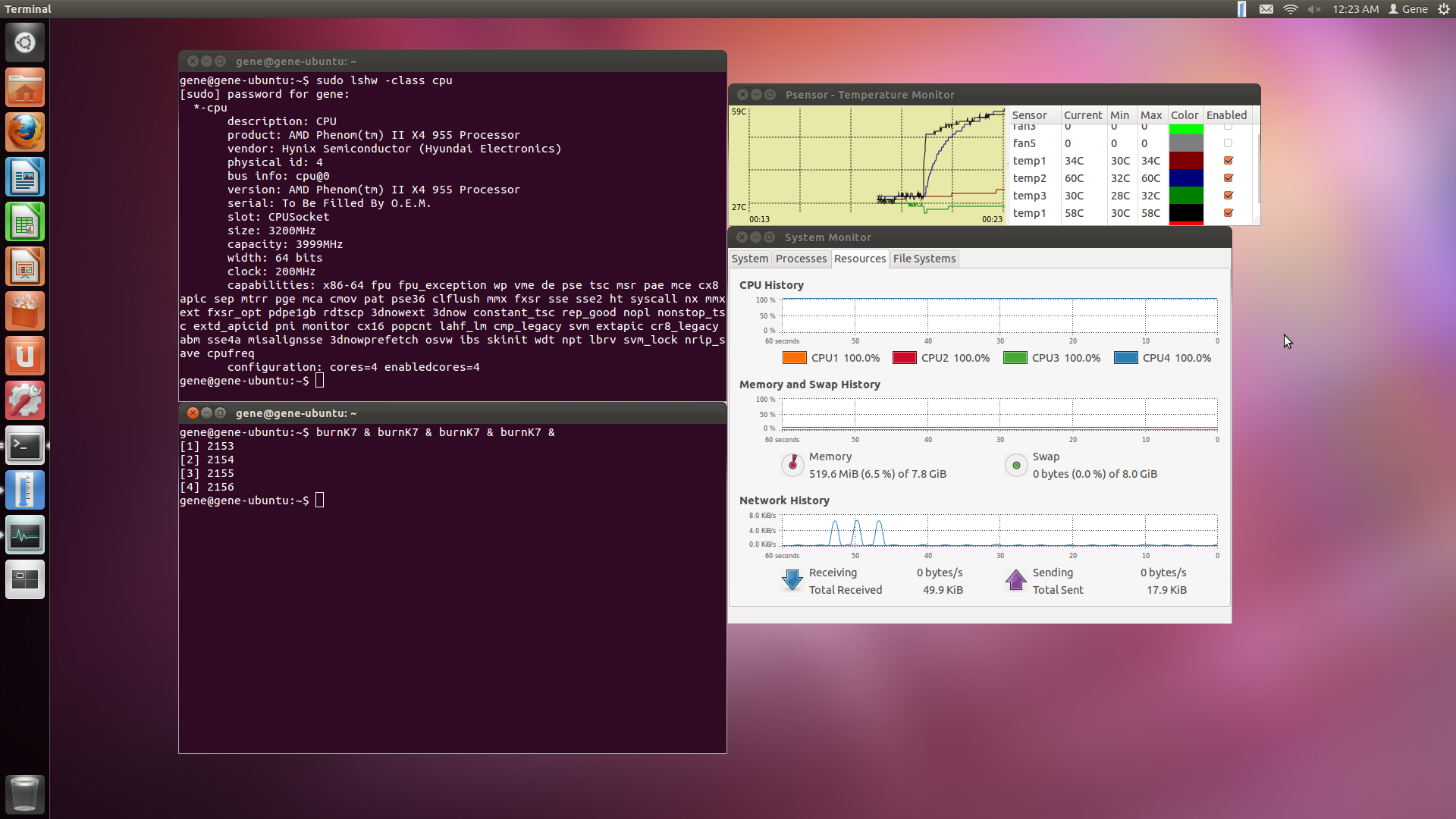
You can see that the maximum temperature was just 46 C – that’s pretty cool for an overclocked processor. I only ran the test for a few minutes because I had been steadily increasing the clock speed little by little to see how far it could go. The test ran comfortably at 3519 MHz, but as soon as I reached 3680 MHz the computer started having issues with booting up. I was able to reach 3841 MHz by increasing the voltage to 1.5 V and 3999 MHz by increasing the voltage to 1.55 V. I was somewhat disappointed because I couldn’t get the clock speed to surpass 4 GHz (as the Phenom II has been pushed to much higher clock speeds with more sophisticated cooling techniques). At this point I couldn’t even run mprime without having my computer crash, but I was able to continue the stress testing by using BurnK7:

Stress testing with BurnK7 at 100% load – 3999 MHz

You can see that the core temperature maxed out at 60 C, so I’m pretty sure I could have pushed it a little further. However, the machine wouldn’t even boot up after I increased the multiplier, so I called it a day. I contacted my friend Daniel Lin (who had been overclocking machines since middle school) with the results, and he responded with his own stress test using an Intel Core i7 quad core:

Daniel Lin’s machine at 4300 MHz

The impressive part is he was able to reach 4300 MHz using nothing but stock voltages (1.32 V) and air cooling. He told me that I had an inferior processor and I believe him (then again, you get what you pay for – the Intel i7 is three times more expensive). If he had liquid cooled his computer he probably could have pushed it even further. Anyway, Daniel told me that you can’t be sure if an overclock is truly stable unless you stress test it over the span of several hours. So, I decided that my next task would be to get Ubuntu’s sensors to output its readings into a text file while I run mprime over the course of 24 hours. I’d also like compare temperature readings depending on whether or not the AC is turned on while I’m away at work. I’ll have the results up next week (hopefully).

Posted in: Logs / Tagged: antec 900, corsair h80, liquid cooling, overclocking

No. 64: Player Piano

3 July, 2012 2:21 AM / Leave a Comment / Gene Dan

Hey everyone,

I started reading Kurt Vonnegut’s Player Piano after I passed C/4 last month. The plot centers around an engineer named Paul Proteus and takes place in an alternative post WW2 era, in which machines have have displaced almost all of human labor. The only jobs left are for engineers, business managers, and hairstylists. As the story progresses, the machines get so good even the engineers end up losing their jobs – hence the title, Player Piano (a Piano that plays music without the need of a human performer). I guess you can see where I’m going with this…I wouldn’t want to spoil the rest, and I haven’t finished the book myself though I’m just 20 pages shy of finishing. Anyway, I became interested in the novel when I was searching the web for articles on post-scarcity economics. The basic idea is that classical economics stems from the conflict between unlimited human wants and limited natural resources. These wants are satisfied through the exchange of goods and services – two or more parties mutually agree to exchange resources – and this is done by valuing one party’s resources against another party’s resources. However, if a society were to achieve the ability to costlessly produce goods and services, the system of exchange and valuation breaks down because you’d no longer be able to value one good relative to another, which makes it impossible for two parties to come to an agreement on how to exchange goods. Some people believe such a system would be more egalitarian since people would no longer have to fight over limited resources. On the other hand, others have hypothesized that such a system would lead not to equality, but to a society dominated by an elite few – the original owners of capital (this is where post-scarcity economics overlaps with Marxist economics).

I’ve thought about such a scenario many times (maybe every other day) but I haven’t been able to reach any solid conclusions over the outcome of this situation. First of all, companies can save costs by automating manual labor and firing workers whose skills have become obsolete. This would result in short term gains because the company would be able to gain market share over its competitors by offering lower prices. However, in order for the company to make money, people would have to be willing to pay for its products. But if such automation were to occur on a large scale, you would end up in a paradoxical situation in which companies would be able to produce goods at no cost – but people wouldn’t be able to buy these goods because they don’t have jobs and aren’t earning wages. Moreover, if these workers aren’t buying goods, then the company won’t make any money. Thus, despite the economy’s ability to produce unlimited goods and services for its people, these people aren’t made any richer because there’s no longer a way to allocate these goods amongst themselves.

Historically, this sort of doomsday scenario hasn’t occurred because automation created more jobs than it destroyed. However, you don’t want to be too careless and assume that automation will continue to create jobs indefinitely just because it has in the past, since there’s no guarantee that this trend of job creation will continue. Perhaps, it might be possible that machines become so effective that they can replace all of human labor…or maybe we’ll eventually get to the point where we can costlessly create humanoid robots that are superior to their biological counterparts, rendering humans obsolete. On the other hand, it might be the case that a post-scarcity society is impossible to achieve. I noticed that in my previous paragraph that the inability to equitably allocate resources amongst a population represents scarcity in service (or scarcity in capital, if you want to take the Marxist point of view). So, while we might not reach post-scarcity, there could be some kind of scenario like “post-human labor”, which would present similar problems.

Anyway, Player Piano is somewhat similar to Zamyatin’s We, and Vonnegut himself said that he “cheerfully ripped off the plot of Brave New World, whose plot had been cheerfully ripped off from Yevgeny Zamyatin’s We.” I read We during the Summer after high school and now that I’m almost done with Player Piano, I can see that the basic structure is similar between the two books, though Vonnegut’s book contains more humor and has a more playful tone than Zamyatin’s. Vonnegut’s book was published in the U.S. after WW2, whereas Zamyatin’s book was written in 1920, suppressed by the Soviets during the Cold War, and later published in 1988. I’d recommend reading both as you’d get to compare the different perspectives between the Soviet Union and the United States, both before the War and afterward.

Posted in: Logs / Tagged: automation, dystopia, post-scarcity economics, vonnegut player piano

No. 63: St. Petersburg Paradox

26 June, 2012 1:32 AM / Leave a Comment / Gene Dan

Hey everyone,

Work has kept me busy, as I’ve spent the last three weeks catching up on the tasks I pushed back while studying for my exam. I didn’t have any time to work on anything creative, so I decided to pull up an old project I had done a year ago on the St. Petersburg Paradox. The St. Petersburg Paradox is a famous problem in mathematics, proposed in 1713 by Nicolas Bernoulli in a letter to fellow mathematician Pierre Raymond de Montmort. The problem consists of a game where the player continuously flips a fair coin until it lands tails. The payout is equal to 2 raised to the number of consecutive heads obtained. For example, if the player gets 1 head, he receives a payout of 2. If he gets 2 heads in a row, he receives a payout of 4. If he gets 3 heads in a row, he receives a payout of 8, and so on and so forth. More formally, we can express the expected payout as:

$latex displaystyle mathrm{E}[mbox{payout}] = sum_{i=1}^infty (mbox{payout for }imbox{ consecutive heads})timesmathrm{Pr}(imbox{ consecutive heads}) $

$latex displaystyle mathrm{E}[mbox{payout}] = sum_i^infty 2^i (.5)^i $

$latex displaystyle = 2timesfrac{1}{2} + 4timesfrac{1}{4} + 8timesfrac{1}{8}cdots $

$latex displaystyle mathrm{E}[mbox{payout}] = 1+1+1cdots = infty$

As you can see, the expected payout is infinite. So, how much would the typical person pay to play this game? It turns out that you might be able to get a person to pay $1 or $5 to play, but once the fee gets into the double-digits, people start getting reluctant. Why is this so? Shouldn’t a rational person be willing to put down any finite amount of money to play the game? That’s why the problem is called the St. Petersburg Paradox. Even though the expected payout is infinite, most people aren’t willing to gamble a large sum of money to play the game.

Intuitively, this makes sense. If you’ve ever tried flipping a penny over and over again, you’ll notice that getting just 5 heads in a row is a rare event. Even then, the payout is just 32. The odds of getting a payout of 1024 is just under one out of a thousand. So, unless you have something better to do than to flip coins all day (and flip them really fast), you’re better off flipping burgers if you want to make a living wage (keep in mind you have to pay each time you play).

I wrote a couple of VBA subroutines to simulate the problem and posted a video of the execution on YouTube, a little more than a year ago (I believe I used a payout of 2^(i-1) instead of 2^i for this simulation):

[youtube=http://www.youtube.com/watch?v=QAizn9gqhO8]

Here, I allow the user to set some values for the simulation, like the game price, starting balance, and number of games. In addition, I added a progress bar, data bars, and sparklines to test out some new features in Excel 2010. The subroutine runs much faster without these features (like a thousand times faster), since the computer gets interrupted each time it has to update the progress bar and spreadsheet features. The columns to the right compare the theoretical distribution to the empirical distribution obtained through the simulation. As you can see, large payouts are very rare, and the player spends most of the time with a negative balance. The important lesson to glean out of this is that it would take a ridiculously large number of games to get a large payout, and relying on expected payouts alone would be a foolish choice to make in a business situation (especially in insurance).

Posted in: Logs, Mathematics / Tagged: st. petersburg paradox, st. petersburg paradox simulation, youtube st. petersburg paradox

No. 62: The Dowry Problem

19 June, 2012 2:30 AM / 1 Comment / Gene Dan

Hey everyone,

Let me introduce you to a famous problem in mathematics. Suppose you’re looking for someone to marry. In order to find that special someone, you, like most people, go on a series of dates, and then pick the best candidate amongst those whom you’ve dated. Unfortunately, while you have the ability to rank the suitors in retrospect, you have no way to determine if your ultimate choice will have been the best one out of all the available options. For example, if you were to pick the 8th person whom you’ve dated as your lifelong partner, until death do you part, you would be able to rank that person amongst the 7 previous candidates, but you would have no idea if anyone better would have come along had you rejected that 8th person and kept looking instead. Hence, the dowry problem. (Also called The Secretary Problem, The Fussy Suitor Problem, The Marriage Problem, The Sultan’s Dowry Problem, The Gogol Game, and The Best Choice Problem).

More formally, suppose you have 100 rankable suitors whom you will date one at a time, in succession. After each date, you have the choice to either reject or accept the suitor. If you accept the suitor, you cannot date anymore candidates and are stuck with that person for life. If you reject the suitor, you will not have the chance to date that candidate again and will move on to the next suitor. With each additional suitor, you have the ability to rank that suitor unambiguously amongst your previous suitors. The process continues until you either accept a suitor, or reject all 100 suitors and doom yourself to a life of lonely bachelorhood or spinsterhood.

So, how do you maximize your chance of selecting the best candidate? It turns out the solution to the problem is to employ an optimal stopping rule. This means you date X number suitors, rank those suitors, and then choose the next suitor who is at least as good as those X suitors. In this problem the optimal stopping rule is to date 37 candidates, and then choose the next suitor who is at least as good as the best of the 37.

It turns out the problem has an elegant solution when n suitors are involved. Generally, the optimal stopping rule is to date n/e (where e is Euler’s constant) candidates, and then choose the next candidate that is at least as good as the the first n/e candidates. This means you should date about 37% of the candidate pool, and then choose the next person who is at least as good as the best of that 37%. So it works no matter how big n is:

100: date the first 37 candidates
1,000: date the first 368 candidates
10,000: date the first 3,679 candidates
100,000: date the first 36,788 candidates
1,000,000: date the first 367,879 candidates

And so on.

I decided to use VBA to run some simulations on this problem to see if I could confirm what we have seen here. Unfortunately, I was not successful, but after looking more carefully, I think I found the problem had to do with the built-in random number generator, as well as the shuffling algorithm I employed to randomize the order of the suitors. I basically generated an array of 100 integers from 1 to 100, shuffled them, applied the stopping rule from 1 to 100, and repeated the procedure to see if the optimal  stopping point (deterimined by the maximum empirical probability of success) matched 37.

As you can see, as the number of iterations increases, the curve approaches that of the true distribution.

After many thousands of iterations I discovered the optimal stopping point centered around 60, and I spent about an hour trying to correct the issue without success. Then I tried counting the proportion of iterations in which the best candidate (integer 100) wound up within the first 33 indices of the array. It turned out that best candidate ended up in the first 33 only 17%-20% of the time, when it ought to be 33%. This would explain why the optimal stopping point for this distribution ended up being further to the right than 100/e. From here I concluded that the shuffling algorithm I used was not shuffling the array uniformly. Here is the code below:

Sub ShuffleArrayInPlace(InArray() As Variant)
''''''''''''''''''''''''''''''''''''''''''''''''''''''''''''''''''''''''''''''''''''
' ShuffleArrayInPlace
' This shuffles InArray to random order, randomized in place.
''''''''''''''''''''''''''''''''''''''''''''''''''''''''''''''''''''''''''''''''''''
Dim N As Long
Dim Temp As Variant
Dim J As Long

Randomize
For N = LBound(InArray) To UBound(InArray)
J = CLng(((UBound(InArray) - N) * Rnd) + N)
If N <> J Then
Temp = InArray(N)
InArray(N) = InArray(J)
InArray(J) = Temp
End If
Next N
End Sub

I obtained the shuffling algorithm from Chip Pearson’s VBA page. I’m willing to give the problem another shot with one that shuffles the array more uniformly, so if anyone can help me out that would be great!

Posted in: Logs, Mathematics / Tagged: best choice problem, fussy suitor problem, marriage problem, simulation, sultan's dowry problem, the secretary problem

Post Navigation

« Previous 1 … 6 7 8 9 10 … 19 Next »

Archives

  • September 2023
  • February 2023
  • January 2023
  • October 2022
  • March 2022
  • February 2022
  • December 2021
  • July 2020
  • June 2020
  • May 2020
  • May 2019
  • April 2019
  • November 2018
  • September 2018
  • August 2018
  • December 2017
  • July 2017
  • March 2017
  • November 2016
  • December 2014
  • November 2014
  • October 2014
  • August 2014
  • July 2014
  • June 2014
  • February 2014
  • December 2013
  • October 2013
  • August 2013
  • July 2013
  • June 2013
  • March 2013
  • January 2013
  • November 2012
  • October 2012
  • September 2012
  • August 2012
  • July 2012
  • June 2012
  • May 2012
  • April 2012
  • March 2012
  • February 2012
  • January 2012
  • December 2011
  • September 2011
  • August 2011
  • July 2011
  • June 2011
  • January 2011
  • December 2010
  • October 2010
  • September 2010
  • August 2010
  • June 2010
  • May 2010
  • April 2010
  • March 2010
  • September 2009
  • August 2009
  • May 2009
  • December 2008

Categories

  • Actuarial
  • Cycling
  • Logs
  • Mathematics
  • MIES
  • Music
  • Uncategorized

Links

Cyclingnews
Jason Lee
Knitted Together
Megan Turley
Shama Cycles
Shama Cycles Blog
South Central Collegiate Cycling Conference
Texas Bicycle Racing Association
Texbiker.net
Tiffany Chan
USA Cycling
VeloNews

Texas Cycling

Cameron Lindsay
Jacob Dodson
Ken Day
Texas Cycling
Texas Cycling Blog
Whitney Schultz
© Copyright 2025 - Gene Dan's Blog
Infinity Theme by DesignCoral / WordPress