• Home
  • Readings
  • Github
  • MIES
  • TmVal
  • About
Gene Dan's Blog

Category Archives: Mathematics

No: 136: MIES – Personal Budget Constraints, Taxes, and Subsidies

2 June, 2020 9:08 PM / 1 Comment / Gene Dan

This entry is part of a series dedicated to MIES – a miniature insurance economic simulator. The source code for the project is available on GitHub.

Current Status

Last week, I demonstrated the first simulation of MIES. Although it can run indefinitely without intervention on my part, I’ve made a lot of assumptions that aren’t particularly realistic – such as the ability of insureds to buy as much insurance as they wanted without any kind of constraint on affordability. I’ll address this today by implementing a budget constraint, a concept typically introduced during the first week of a second year economics course.

Most of the economic theory that I’ll be introducing to MIES for the time being comes from two books: Hal Varian’s Intermediate Microeconomics, a favorite of mine from school, and Zweifel and Eisen’s Insurance Economics, which at least according to the table of contents and what little I’ve read so far, seems to have much of the information I’d want to learn about for MIES.

I’m going to avoid repeating much of what can already be read in these books, so just an fyi, these are the sources I’m drawing from. My goals are to refresh my knowledge of economics as I read and then implement what I see in Python to add features to MIES.

The Economics Module

I’ve added a new module to the project, econtools.py. For now, this will contain the classes for exploring economics concepts with MIES, but seeing how much it has grown in just one week, it’s likely I’ll break it up in the near future. I’ll go over the first classes I’ve written for the module, those written for the budget constraint: Budget, Good, Tax, and Subsidy.

Budget Constraint

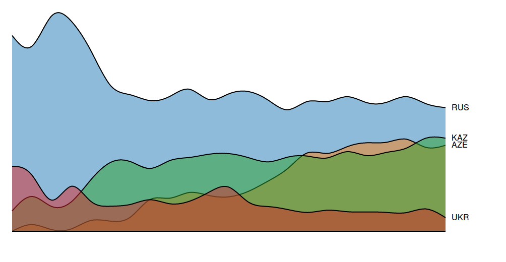
Those of you who have taken an economics course ought to find the following graph, a budget constraint, familiar:

As in the real world, there are only two goods that a person can possibly buy:

  1. Insurance
  2. Non-insurance

The budget constraint represents the set of possible allocations between insurance and non-insurance, aka all other goods. This can be represented by an equation as well:

    \[p_1 x_1 + p_2 x_2 = m\]

Where each x represents the quantity of each good and each p represents the prices per unit for each good, and m represents income. People can only buy as much insurance as their incomes can support, hence the need for introducing this constraint into MIES for each person. The budget constraint simply shows that in order to buy one dollar more of insurance, you have to spend one dollar less on anything else that you were going to buy with your income.

The price of insurance is often thought of as a rate per unit of exposure, exposure being some kind of denominator to measure risk, such as miles driven, house-years, actuarial exams taken, or really anything you can think of that correlates with a risk that you’d like to charge money for.

Interestingly, there is nothing in the budget constraint as shown above that would prevent someone from insuring something twice or purchasing some odd products like a ‘lose-1-dollar-get-5-dollars back’ multiplier scheme. I’m not sure if these are legal or simply just discouraged by insurers as I’ve never tried to buy such a product myself or seen it advertised. I could imagine why insurers would not to sell these things – maybe due to the potential for fraud or the fact that an insured thing is 100% correlated with itself. On the other hand, a company might be able to compensate for these risks by simply charging more money to accept them. Regardless, if these products are really undesirable, I’d rather let the simulations demonstrate the impact of unrestricted product design than to have it constrained from the start. I’ll save that for another day.

The budget constraint is modeled with the Budget class in econtools.py. It accepts the goods to be allocated along with other relevant information, such as their prices and the income of the person for whom we are modeling the budget. You’ll see that the class contains references to the other component classes (Good, Tax, Subsidy) which are explained later:

Python
1
2
3
4
5
6
7
8
9
10
11
12
13
14
15
16
17
18
19
20
21
22
23
24
25
26
27
28
29
30
31
32
33
34
35
36
37
38
39
40
41
42
43
44
45
46
47
48
49
50
51
52
53
54
55
56
57
58
59
60
61
62
63
64
65
66
67
68
69
70
71
72
73
74
75
76
77
78
79
80
81
82
83
84
85
86
87
88
89
90
91
92
93
94
95
96
97
98
99
100
101
102
103
104
105
106
107
108
109
110
111
112
113
114
115
116
117
118
119
120
121
122
123
124
125
126
127
128
129
130
131
132
133
134
135
136
137
138
class Budget:
    def __init__(self, good_x, good_y, income, name):
        self.good_x = good_x
        self.good_y = good_y
        self.income = income
        self.x_lim = self.income / (min(self.good_x.adjusted_price, self.good_x.price)) * 1.2
        self.y_lim = self.income / (min(self.good_y.adjusted_price, self.good_y.price)) * 1.2
        self.name = name
 
    def get_line(self):
        data = pd.DataFrame(columns=['x_values', 'y_values'])
        data['x_values'] = np.arange(int(min(self.x_lim, self.good_x.ration)) + 1)
 
        if self.good_x.tax:
            data['y_values'] = self.calculate_budget(
                good_x_price=self.good_x.price,
                good_y_price=self.good_y.price,
                good_x_adj_price=self.good_x.adjusted_price,
                good_y_adj_price=self.good_y.adjusted_price,
                m=self.income,
                modifier=self.good_x.tax,
                x_values=data['x_values']
            )
        elif self.good_x.subsidy:
            data['y_values'] = self.calculate_budget(
                good_x_price=self.good_x.price,
                good_y_price=self.good_y.price,
                good_x_adj_price=self.good_x.adjusted_price,
                good_y_adj_price=self.good_y.adjusted_price,
                m=self.income,
                modifier=self.good_x.subsidy,
                x_values=data['x_values']
            )
        else:
            data['y_values'] = (self.income / self.good_y.adjusted_price) - \
                       (self.good_x.adjusted_price / self.good_y.adjusted_price) * data['x_values']
 
        return {'x': data['x_values'],
                'y': data['y_values'],
                'mode': 'lines',
                'name': self.name}
 
    def calculate_budget(
            self,
            good_x_price,
            good_y_price,
            good_x_adj_price,
            good_y_adj_price,
            m,
            modifier,
            x_values
    ):
        y_int = m / good_y_price
        slope = -good_x_price / good_y_price
        adj_slope = -good_x_adj_price / good_y_adj_price
        base_lower = int(modifier.base[0])
        base_upper = int(min(modifier.base[1], max(m / good_x_price, m / good_x_adj_price)))
        modifier_type = modifier.style
 
        def lump_sum(x):
            if x in range(modifier.amount + 1):
                x2 = y_int
                return x2
            else:
                x2 = y_int + adj_slope * (x - modifier.amount)
                return x2
 
        def no_or_all_adj(x):
            x2 = y_int + adj_slope * x
            return x2
 
        def beg_adj(x):
            if x in range(base_lower, base_upper + 1):
                x2 = y_int + adj_slope * x
                return x2
            else:
                x2 = y_int + slope * (x + (adj_slope/slope - 1) * base_upper)
                return x2
 
        def mid_adj(x):
            if x in range(base_lower):
                x2 = y_int + slope * x
                return x2
            elif x in range(base_lower, base_upper + 1):
                x2 = y_int + adj_slope * (x + (slope/adj_slope - 1) * (base_lower - 1))
                return x2
            else:
                x2 = y_int + slope * (x + (adj_slope/slope - 1) * (base_upper - base_lower + 1))
                return x2
 
        def end_adj(x):
            if x in range(base_lower):
                x2 = y_int + slope * x
                return x2
            else:
                x2 = y_int + adj_slope * (x + (slope/adj_slope - 1) * (base_lower - 1))
                print(x, x2)
                return x2
 
        cases = {
            'lump_sum': lump_sum,
            'no_or_all': no_or_all_adj,
            'beg_adj': beg_adj,
            'mid_adj': mid_adj,
            'end_adj': end_adj,
        }
 
        if modifier_type == 'lump_sum':
            option = 'lump_sum'
        elif modifier.base == [0, np.Inf]:
            option = 'no_or_all'
        elif (modifier.base[0] == 0) and (modifier.base[1] < max(m/good_x_price, m/good_x_adj_price)):
            option = 'beg_adj'
        elif (modifier.base[0] > 0) and (modifier.base[1] < max(m/good_x_price, m/good_x_adj_price)):
            option = 'mid_adj'
        else:
            option = 'end_adj'
 
        adj_func = cases[option]
        print(option)
        return x_values.apply(adj_func)
 
    def show_plot(self):
        fig = go.Figure(data=go.Scatter(self.get_line()))
        fig['layout'].update({
            'title': 'Budget Constraint',
            'title_x': 0.5,
            'xaxis': {
                'range': [0, self.x_lim],
                'title': 'Amount of ' + self.good_x.name
            },
            'yaxis': {
                'range': [0, self.y_lim],
                'title': 'Amount of ' + self.good_y.name
            },
            'showlegend': True
        })
        plot(fig)

Goods

The Good class represents things consumers can buy. We can set the price, as well as apply any taxes and subsidies:

1
2
3
4
5
6
7
8
9
10
11
12
13
14
15
16
17
18
19
20
21
22
23
24
25
26
27
28
29
30
31
32
33
34
35
36
37
38
class Good:
    def __init__(
        self,
        price,
        tax=None,
        subsidy=None,
        ration=None,
        name='Good',
    ):
 
        self.price = price
        self.tax = tax
        self.subsidy = subsidy
        self.adjusted_price = self.apply_tax(self.price)
        self.adjusted_price = self.apply_subsidy(self.adjusted_price)
        if ration is None:
            self.ration = np.Inf
        else:
            self.ration = ration
        self.name = name
 
    def apply_tax(self, price):
        if (self.tax is None) or (self.tax.style == 'lump_sum'):
            return price
        if self.tax.style == 'quantity':
            return price + self.tax.amount
        # else, assume ad valorem
        else:
            return price * (1 + self.tax.amount)
 
    def apply_subsidy(self, price):
        if (self.subsidy is None) or (self.subsidy.style == 'lump_sum'):
            return price
        if self.subsidy.style == 'quantity':
            return price - self.subsidy.value
        # else, assume ad valorem
        else:
            return price * (1 - self.subsidy.amount)

Taxes

Taxes can be added to goods via the Tax class:

Python
1
2
3
4
5
class Tax:
    def __init__(self, amount, style, base=None):
        self.amount = amount
        self.style = style
        self.base = base

The tax class has three attributes, the amount, which specifies the amount of tax to be applied, style, which (for lack of a better word) specifies whether the tax is a quantity, value (or ad valorem) tax, or lump-sum tax. A quantity tax is a fixed amount of tax applied to each unit of a good purchased, a value tax is a tax that is proportional to the price of a good, and a lump-sum tax is a one-time tax paid for participating in the market for that good. Finally, the base attribute specifies over what quantities a tax applies (for example, a tax applied to the first 5 units purchased).

To demonstrate, we’ll add three different types of taxes to our insurance, first by specifying the tax details, and then adding them to the goods, we then specify the relevant budget constraints:

Python
1
2
3
4
5
6
7
8
9
10
11
12
13
14
15
16
17
18
19
20
ad_valorem_tax = ec.Tax(amount=1, style='value', base=[0,np.Inf])
quantity_tax = ec.Tax(amount=4, style='quantity', base=[0, np.Inf])
all_other = ec.Good(price=1, name='All Other Goods')
ad_valorem_first_two = ec.Tax(amount=1, style='value', base=[0, 2])
 
insurance_no_tax = ec.Good(price=1, name='Insurance')
insurance_ad_valorem = ec.Good(price=1, tax=ad_valorem_tax, name='Insurance')
insurance_value = ec.Good(price=1, tax=quantity_tax, name='Insurance')
insurance_first_two = ec.Good(price=1, tax=ad_valorem_first_two, name='Insurance')
 
budget_no_tax = ec.Budget(insurance_no_tax, all_other, income=10, name='No Tax')
budget_ad_valorem = ec.Budget(insurance_ad_valorem, all_other, income=10, name='Ad Valorem Tax')
budget_quantity = ec.Budget(insurance_value, all_other, income=10, name='Value Tax')
budget_first_two = ec.Budget(insurance_first_two, all_other, income=10, name='Ad Valorem Tax - First 2')
 
fig = go.Figure()
fig.add_trace(go.Scatter(budget_no_tax.get_line()))
fig.add_trace(go.Scatter(budget_ad_valorem.get_line()))
fig.add_trace(go.Scatter(budget_quantity.get_line()))
fig.add_trace(go.Scatter(budget_first_two.get_line()))

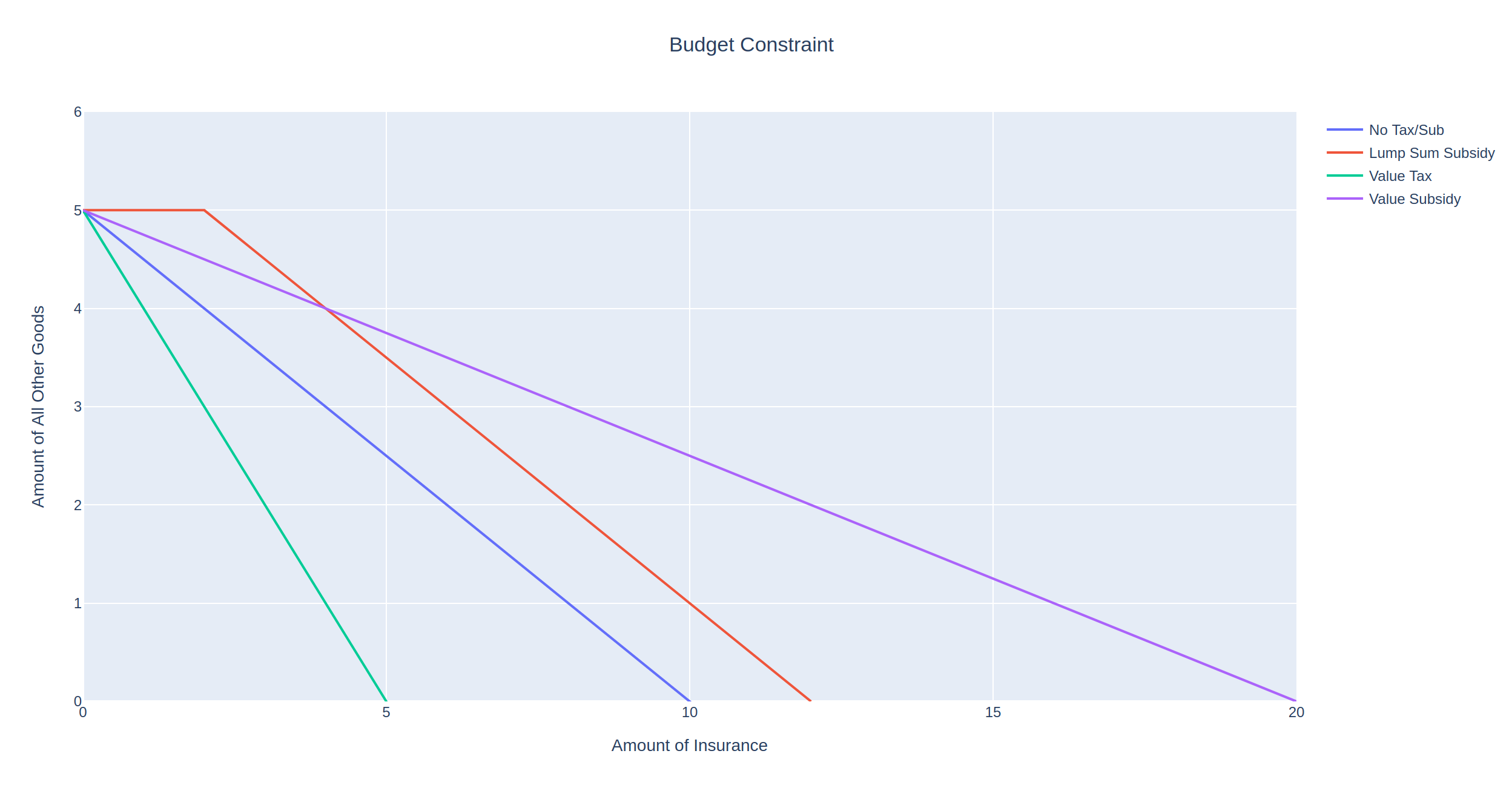
We can now plot the resulting budget constraints on a single graph:

As expected, the no-tax scenario (blue line) allows the insured to purchase the most insurance, indicated by the x-intercept at 10. Contrast this with the most punitive tax, the value tax shown by the green line with an x-intercept at 2. In this scenario, we increase the price of each unit of insurance form 1 to 5, so that the insured can at most afford 2 units of insurance.

Between these two extremes are the two ad valorem taxes that double the price of insurance. However, the purple line is less punitive as it only taxes the first two units of insurance purchased.

Subsidies

Subsidies behave very similarly to taxes, so much so that I have considered either defining them as a single class or both inheriting from a superclass. Instead of penalizing the consumer, subsidies reward the consumer either by lowering the price of a good or by giving away free units of a good:

Python
1
2
3
4
5
class Subsidy:
    def __init__(self, amount, style, base=None):
        self.amount = amount
        self.style = style
        self.base = base

Just like with taxes, we can specify the subsidy amount, style, and quantities to which it applies. For instance, let’s suppose that as part of a risk-management initiative, the government grants 2 free units of insurance to a consumer in the form of a lump sum subsidy:

The subsidy has allowed the consumer to have at least 2 units of insurance without impacting the maximum amount of all other goods they can buy. We also see that the maximum amount of insurance the consumer can purchase has increased by the same amount, from 10 to 12.

MIES Integration

To integrate these classes and make use of the econtools.py module, I’ve made some changes to the existing MIES modules. In last week’s example, income was irrelevant for each person, and therefore they were unconstrained with respect to the amount of insurance they could purchase. Since a budget constraint is only relevant in the form of some kind of limited spending power, I’ve decided to introduce consumer income into MIES.

Income is now determined by a Pareto distribution, though certainly other distributions are possible and more realistic. In the parameters.py module, I’ve added a value of 30000 as the scale parameter for each person:

Python
1
2
3
4
5
6
7
person_params = {
    'age_class': ['Y', 'M', 'E'],
    'profession': ['A', 'B', 'C'],
    'health_status': ['P', 'F', 'G'],
    'education_level': ['H', 'U', 'P'],
    'income': 30000
}

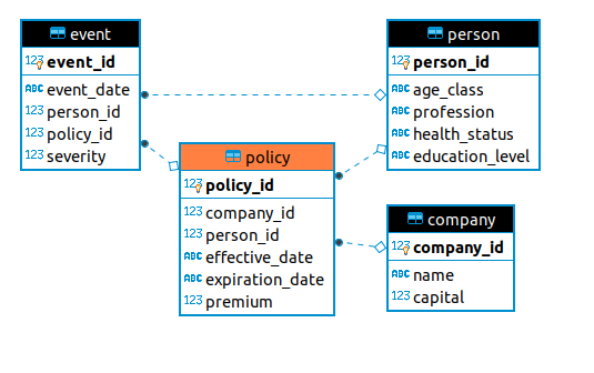
The person SQLite table has also been updated to accept income as a field:

Python
1
2
3
4
5
6
7
8
9
10
11
12
13
14
15
16
17
18
19
20
21
22
23
24
25
26
27
28
29
30
31
32
33
34
35
36
class Person(Base):
    __tablename__ = 'person'
 
    person_id = Column(
        Integer,
        primary_key=True
    )
    age_class = Column(String)
    profession = Column(String)
    health_status = Column(String)
    education_level = Column(String)
    income = Column(Float)
 
    policy = relationship(
        "Policy",
        back_populates="person"
    )
    event = relationship(
        "Event",
        back_populates="person"
    )
 
    def __repr__(self):
        return "<Person(" \
               "age_class='%s', " \
               "profession='%s', " \
               "health_status='%s', " \
               "education_level='%s'" \
               "income='%s'" \
               ")>" % (
                self.age_class,
                self.profession,
                self.health_status,
                self.education_level,
                self.income
                )

And finally, I’ve added a method to the environment class to assign incomes to each person by drawing from the Pareto distribution using the scale parameter:

Python
1
2
3
4
5
6
7
8
9
10
11
12
13
14
15
16
17
18
19
20
21
22
23
24
25
26
27
28
29
30
31
32
33
    def make_population(self, n_people):
        age_class = pm.draw_ac(n_people)
        profession = pm.draw_prof(n_people)
        health_status = pm.draw_hs(n_people)
        education_level = pm.draw_el(n_people)
        income = pareto.rvs(
            b=1,
            scale=pm.person_params['income'],
            size=n_people,
        )
 
        population = pd.DataFrame(list(
            zip(
                age_class,
                profession,
                health_status,
                education_level,
                income
            )
        ), columns=[
            'age_class',
            'profession',
            'health_status',
            'education_level',
            'income'
        ])
 
        population.to_sql(
            'person',
            self.connection,
            index=False,
            if_exists='append'
        )

This results in a mean income of five figures with some high-earning individuals making a few million dollars per year. To examine the budget constraint for a single person in MIES, we can do so by running two iterations of the simulation and then querying the database:

Python
1
2
3
4
5
6
7
8
9
10
11
12
13
14
15
16
17
18
19
20
21
22
23
24
25
26
27
28
29
30
31
32
33
34
35
36
37
38
39
40
import pandas as pd
import datetime as dt
import sqlalchemy as sa
import econtools as ec
from SQLite.schema import Person, Policy, Base, Company, Event
from sqlalchemy.orm import sessionmaker
from entities import God, Broker, Insurer
import numpy as np
import plotly.graph_objects as go
from plotly.offline import plot
 
 
pd.set_option('display.max_columns', None)
 
 
engine = sa.create_engine('sqlite:///MIES_Lite.db', echo=True)
Session = sessionmaker(bind=engine)
Base.metadata.create_all(engine)
 
gsession = Session()
 
 
ahura = God(gsession, engine)
ahura.make_population(1000)
 
pricing_date = dt.date(1, 12, 31)
 
 
rayon = Broker(gsession, engine)
company_1 = Insurer(gsession, engine, 4000000, Company, 'company_1')
company_1_formula = 'severity ~ age_class + profession + health_status + education_level'
pricing_status = 'initial_pricing'
free_business = rayon.identify_free_business(Person, Policy, pricing_date)
companies = pd.read_sql(gsession.query(Company).statement, engine.connect())
 
rayon.place_business(free_business, companies, pricing_status, pricing_date, company_1)
ahura.smite(Person, Policy, pricing_date + dt.timedelta(days=1))
company_1.price_book(Person, Policy, Event, company_1_formula)
pricing_status = 'renewal_pricing'
rayon.place_business(free_business, companies, pricing_status, pricing_date, company_1)

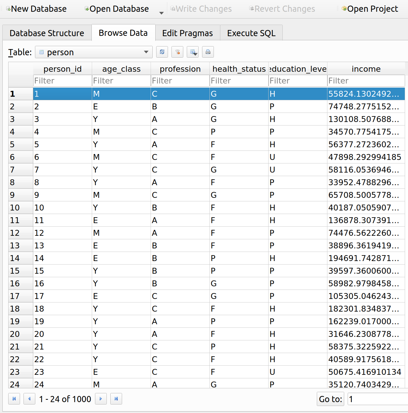
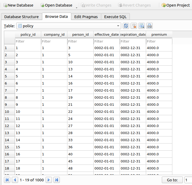
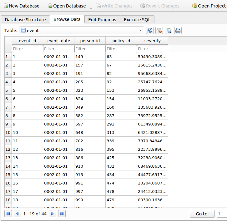
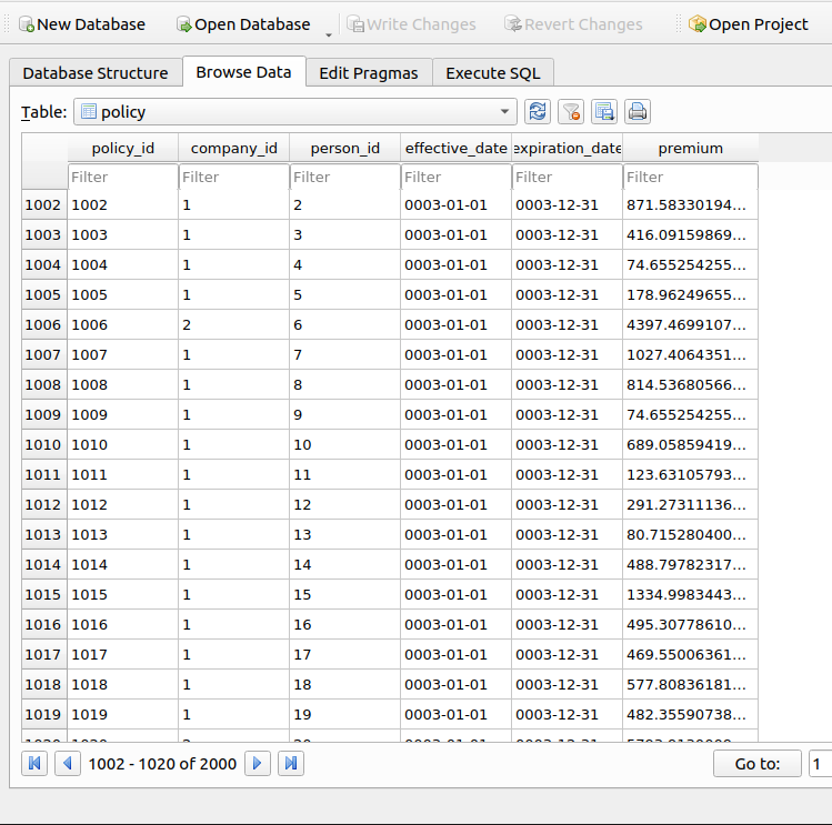
When we query the person table, we can see that the person we are interested in (id=1) has an income of about 56k per year:

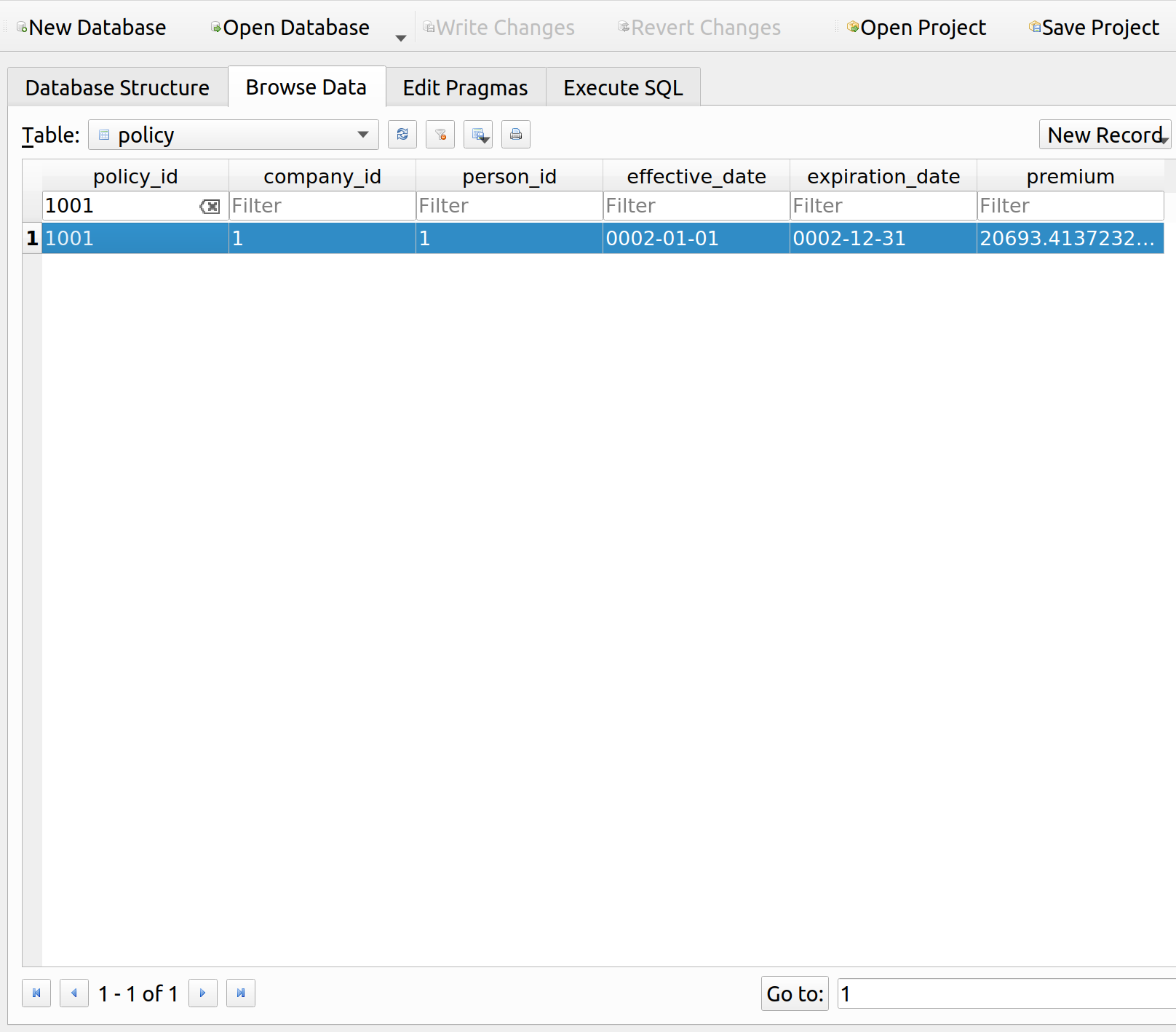
We can also see that their premium upon renewal was about 21k, almost half their income and much higher than the original premium of 4k:

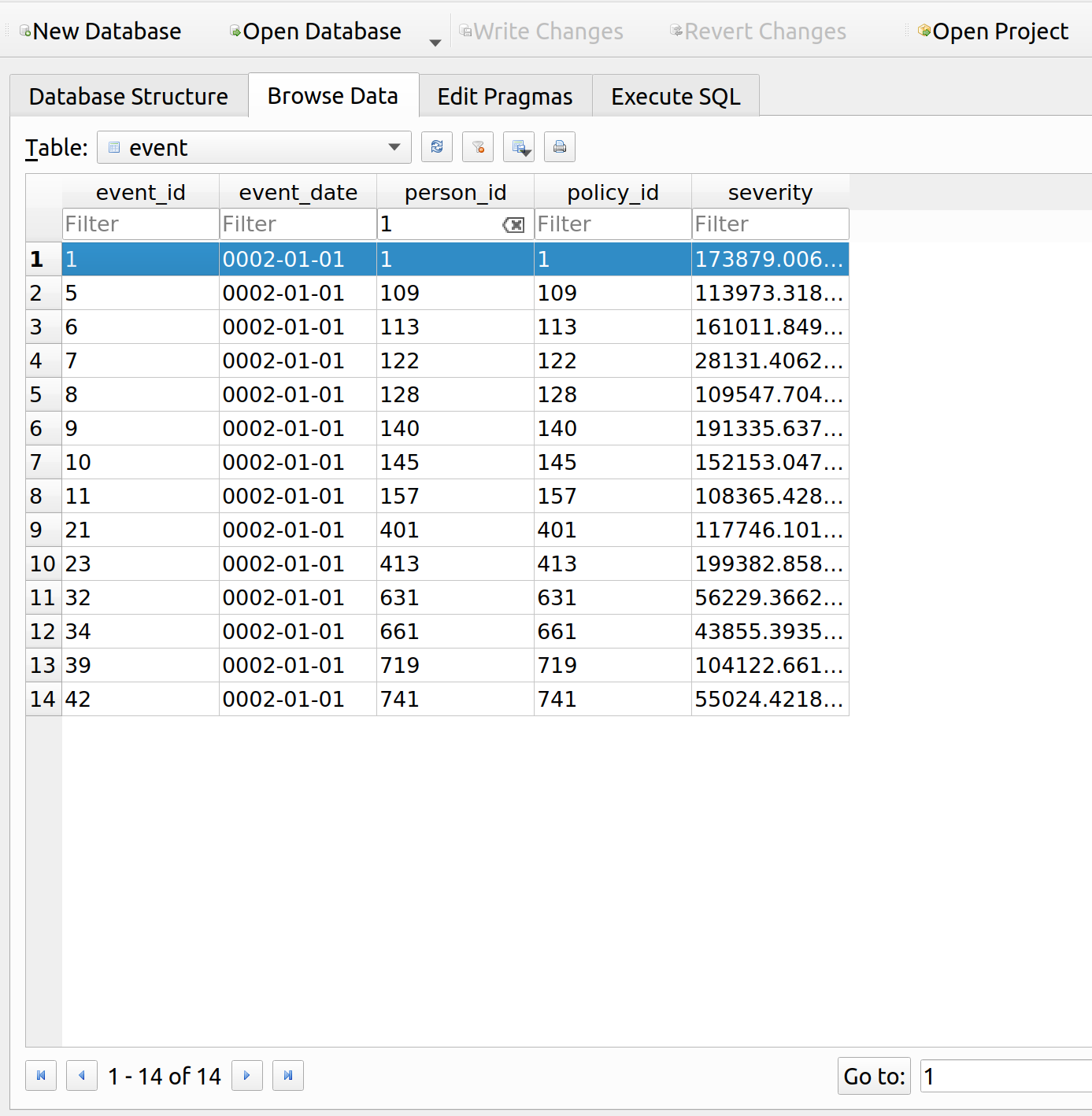
Let’s look at the events table to see why their premium is so high. It looks like they had a loss of about 174k, so the insurance up to this point has at least been worth their while:

We can now query the relevant information about this person, and use econtools.py to graph their budget constraint prior to and during renewal:

Python
1
2
3
4
5
6
7
8
9
10
11
12
13
14
15
16
17
18
19
20
21
22
23
24
25
26
27
28
29
30
31
32
33
34
35
36
37
38
39
40
41
42
43
44
45
46
47
48
49
myquery = gsession.query(Person.person_id, Person.income, Policy.policy_id, Policy.premium).\
    outerjoin(Policy, Person.person_id == Policy.person_id).\
    filter(Person.person_id == str(1)).\
    filter(Policy.policy_id == str(1001))
 
my_person = pd.read_sql(myquery.statement, engine.connect())
 
my_person
 
all_other = ec.Good(price=1, name="All Other Goods")
price = my_person['premium'].loc[0]
id = my_person['person_id'].loc[0]
income = my_person['income'].loc[0]
renewal = ec.Good(price=price, name="Insurance")
 
original = ec.Good(price=4000, name="Insurance")
budget_original = ec.Budget(good_x=original, good_y=all_other, income=income, name='Orginal Budget')
renewal_budget = ec.Budget(good_x=renewal, good_y=all_other, income=income, name='Renewal Budget')
 
fig = go.Figure()
fig.add_trace(go.Scatter(budget_original.get_line()))
fig.add_trace(go.Scatter(renewal_budget.get_line()))


fig['layout'].update({
            'title': 'Budget Constraint',
            'title_x': 0.5,
            'xaxis': {
                'range': [0, 20],
                'title': 'Amount of Insurance'
            },
            'yaxis': {
                'range': [0, 60000],
                'title': 'Amount of All Other Goods'
            },
            'showlegend': True,
            'legend': {
                'x': .71,
                'y': 1
            },
            'width': 590,
            'height': 450,
            'margin': {
                'l':10
            }
        })
 
fig.write_html('mies_budget.html', auto_open=True)

This insured used to be able to afford about 14 units of insurance prior to their large claim. Upon renewal, their premium went up drastically which led to a big drop in affordability, as indicated by the red line. Now they can only afford a little more than 2 units of insurance.

Further Improvements

The concept of utility builds upon the budget constraint by answering the question – given a budget, what is the optimal allocation of goods one can purchase? I think this will be a bit harder and may take some time to program. As I’ve worked on this, I’ve found my programming stints to fall into three broad categories:

  1. Economic Theory
  2. Insurance Operations
  3. Refactoring

Every now and then after adding stuff to MIES, the code will get messy and the object dependencies more complex than they need to be, therefore, I ought to spend a week here or there just cleaning up the code. Sometimes I’ll stop to work on some practice problems to strengthen my theoretical knowledge, which I suspect I’ll need to do soon since I need a refresher on partial derivatives, which are used to find optimal consumption bundles.

Posted in: Actuarial, Mathematics, MIES

No. 135: MIES – Simulating an Insurance Market

25 May, 2020 7:02 PM / Leave a Comment / Gene Dan

MIES, which stands for miniature insurance economic simulator, is a model of the insurance industry. during the course of my actuarial studies, I’ve been introduced to various concepts such as pricing, reserving, capital management, and regulation. While each topic made sense within the scope of the paper in which it was discussed, I never had a tool that I could use to put all the concepts together to get a cohesive narrative on their aggregate impact on the economy – that is, not just the impact on my employer (or department), but upon the insureds, other insurers, the uninsured, and the government. This has been my long-running attempt at making this tool.

I thought about making this many years ago, but soon discovered that I would need quite a lot of working experience as well as knowledge of various technologies. One thing I wanted to do was to represent each entity in the insurance sector as a class in object-oriented programming, which languages like R weren’t well-suited for. However, I’ve gotten the chance to use a lot of Python over the last few months and felt confident to put together my first self-sustaining simulation – as in, a simulation where policy issuance, pricing, and claims handling would happen in a self-sustaining cycle. This is what I’ll discuss today. As I continue to comb through literature and learn additional skills, I’ll gradually incorporate new aspects of the insurance industry into the model and relax assumptions to make things more realistic.

I’ve also developed the early versions of a few useful methods that were inspired by the slow-running processes I’ve often encountered on the job. For example, the function in_force() lets me, within a single line of code, return the entire in-force book for a business on any date. Believe it or not, what sounds like a straightforward request can take many days or even require a multi-month project at a real insurance company if the backend infrastructure is not built appropriately (in this particular scenario it’s not that writing the function is hard, but moreso dealing with something like a collection of incompatible databases left over from a long string of mergers and acquisitions – I hope other actuaries sympathize with me here). While I’ve applied this method on a highly simplified database, I just hope it gives some amount of motivation for anyone reading on what may be possible, if they’ve ever encountered a similar slow-running process at their own job.

Project Structure

As of today, the project contains four core modules that interact with each other to drive the simulations.

  1. schema.py
  2. Contains the ORM equivalent of the data definition language used to create the underling SQLite tables and define their relationships.

  3. parameters.py
  4. Contains the population characteristics from which the random variable parameters are derived.

  5. entities.py
  6. Contains the OOP representations of players in the insurance market, i.e., insurers, brokers, and customers.

  7. simulation.py
  8. Used to run the simulation, drawing objects from the other three modules.

Database Schema – SQLAlchemy/SQLite

The current database consists of a SQLite file. While I had previously mentioned that I would eventually like to have MIES running on postgres, using SQLite has made it easier for me to pursue rapid prototyping of various schemas without the cumbersome configuration process that comes with the postgres installation or other production-grade database management systems. SQLite does come with its disadvantages – for instance, it’s not quite as good with concurrency control or authorization in a multi-user environment.

One tool that I have been using to define and interact with the database file is SQLAlchemy, an object-relational mapper between Python and SQL. SQLAlchemy allows me to define and query the underlying MIES database without having to write any SQL. An object relational mapping is a framework used to reconcile a problem known as the object-relational impedance mismatch. The relational database model strives to achieve what’s known as program-data independence, that is, changes in the underlying data should not force changes in the software that depend on that data. On the other hand, in object-oriented programming languages like Python, data and the programs that manipulate that data are intricately linked, so trying to use SQL and Python together tends to break that independence. Therefore, an ORM tool like SQLAlchemy inserts a layer between the conflicting paradigms so as to minimize the disruption to the programs whenever the data change. Should the data change, you could update the mapping instead of having to update all the Python programs that depend on the data.

I have read varying opinions on the use of ORMs, but I have found writing embedded SQL queries, whether in R or Python, to be quite cumbersome, so I’ve decided to give SQLAlchemy a shot to see if I’d be more comfortable manipulating database tables as Python classes. I’ve liked it so far, although the learning curve can be steep, and more effort is required upfront to carefully define the schema and the relationships within it before you can query it with the ORM.

The database currently consists of a single SQLite file representing the entire insurance market. Once I learn how to implement multiple schemas and sessions within the simulation, it is my intention to split it up into multiple databases so that each entity (environment, brokers, insurers, etc.) receives its own database, which is closer to what you’d see in the real world. However, I’ve programmed the insurers in such a way that they cannot access each other’s data and can only build predictive models using their own book, so we should be okay for the limited applications that I’ve introduced in this early version.

The following image shows the current ER diagram of the environment, consisting of four tables:

  1. person
  2. Represents the population and personal characteristics of the potential insureds.

  3. company
  4. Represents the insurance companies involved in the marketplace.

  5. policy
  6. Represents the policies written in the market. Each company can only access its own insureds.

  7. event
  8. Represents fortuitous events that can happen to people.

Person

While these tables can be created with a variety of tools, such as SQL data definition language (DDL), or ER diagramming software (for those preferring a GUI), SQLAlchemy lets us create them entirely in Python. Below, the person table is represented by the Person class, within which we specify its columns and relationships with other tables:

The Person class in schema.py
Python
1
2
3
4
5
6
7
8
9
10
11
12
13
14
15
16
17
18
19
20
21
22
23
24
25
26
27
28
29
30
31
32
33
34
35
36
37
38
39
40
41
from sqlalchemy.ext.declarative import declarative_base
from sqlalchemy import Column, Integer, String, Date, Float
from sqlalchemy import ForeignKey
from sqlalchemy.orm import relationship
 
Base = declarative_base()
 
 
class Person(Base):
    __tablename__ = 'person'
 
    person_id = Column(
        Integer,
        primary_key=True
    )
    age_class = Column(String)
    profession = Column(String)
    health_status = Column(String)
    education_level = Column(String)
 
    policy = relationship(
        "Policy",
        back_populates="person"
    )
    event = relationship(
        "Event",
        back_populates="person"
    )
 
    def __repr__(self):
        return "<Person(" \
               "age_class='%s', " \
               "profession='%s', " \
               "health_status='%s', " \
               "education_level='%s'" \
               ")>" % (
                self.age_class,
                self.profession,
                self.health_status,
                self.education_level
                )

Each person in the market is identified by the unique identifier person_id, and are characterized by their age, profession, health status, and education level, which are dynamically generated for each simulation. This table has two relationships, one to the policy table, and another to the event table.

Policy

The policy table contains information for each policy, such as effective date, expiration date, premium, and company. This is the central table in the database, linking people, company, and insured events together:

Python
1
2
3
4
5
6
7
8
9
10
11
12
13
14
15
16
17
18
19
20
21
22
23
24
25
26
27
28
29
30
31
32
33
34
35
36
37
38
39
40
41
42
class Policy(Base):
    __tablename__ = 'policy'
 
    policy_id = Column(
        Integer,
        primary_key=True
    )
    company_id = Column(
        Integer,
        ForeignKey('company.company_id')
    )
    person_id = Column(
        Integer,
        ForeignKey('person.person_id')
    )
    effective_date = Column(Date)
    expiration_date = Column(Date)
    premium = Column(Float)
 
    company = relationship(
        "Company",
        back_populates="policy"
    )
    person = relationship(
        "Person",
        back_populates="policy"
    )
    event = relationship(
        "Event",
        back_populates="policy"
    )
 
    def __repr__(self):
        return "<Policy(person_id ='%s'," \
               "effective_date ='%s', " \
               "expiration_date='%s', " \
               "premium='%s')>" % (
                self.person_id,
                self.effective_date,
                self.expiration_date,
                self.premium
                )

Event

The event table contains fortuitous, financially damaging events that may happen to people. For this simulation, each event and person is insured, so there is no distinction between a claim and an event. Future simulations will relax those assumptions as not all risks are insured in the real world:

Python
1
2
3
4
5
6
7
8
9
10
11
12
13
14
15
16
17
18
19
20
21
22
23
24
25
26
class Event(Base):
    __tablename__ = 'event'
 
    event_id = Column(
        Integer,
        primary_key=True
    )
    event_date = Column(Date)
    person_id = Column(
        Integer,
        ForeignKey('person.person_id')
    )
    policy_id = Column(
        Integer,
        ForeignKey('policy.policy_id')
    )
    severity = Column(Float)
 
    person = relationship(
        "Person",
        back_populates="event"
    )
    policy = relationship(
        "Policy",
        back_populates="event"
    )

Company

The final table in the database contains company information. So far, the only important column is the identifier, which the company can use to determine a pricing model. You’ll see a definition for starting capital which will be used in future simulations to model profitability and return on capital, but for now it is unused:

Python
1
2
3
4
5
6
7
8
9
10
11
12
13
14
15
16
17
18
19
20
21
22
23
class Company(Base):
    __tablename__ = 'company'
 
    company_id = Column(
        Integer,
        primary_key=True
    )
    name = Column(String)
    capital = Column(Float)
 
    policy = relationship(
        "Policy",
        back_populates="company"
    )
 
    def __repr(self):
        return "<Company(" \
               "name='%s'," \
               " capital='%s'" \
               ")>" % (
                self.name,
                self.capital
                )

If you look at the actual schema file in the GitHub repository, you’ll notice there’ also a table for claims. This has no use at the moment, but will in future versions once I start to differentiate between events and claims.

Simulation Parameters

One of the goals I prioritized for this version was to get a self-sustaining simulation running, which meant I made many simplifying assumptions to reduce the complexity of technical things I had to learn (such as multi-processing, multiple sessions, concurrency, time-based mathematics, etc.). These include:

  1. Each iteration of the simulation begins on the last day of a calendar year.
  2. All policies are effective on the following day, last for one year, and expire on the day of the next iteration.
  3. All events happen on the first day policies become effective.
  4. All events are covered, and are reported and paid immediately. There is no loss development.
  5. Companies do not go bankrupt, and can exist indefinitely.
  6. Each company can only develop pricing models on the business they have written.
  7. During renewals, each person will simply choose the insurer that offers the lowest premium.
  8. There are no policy expenses.

There are more assumptions, but these are the most obvious ones that I could think of. The parameters module in the repository contains values attached to each person’s characteristics, such as age class, stored in dictionaries. There is nothing particularly special about these values other than that they lead to five- to six-figure claim amounts, which are common in insurance. These values are used to generate parameters for the probability distributions that are used to generate event losses. These distributions are Poisson for event frequency and gamma for loss value:

Python
1
2
3
4
5
6
7
8
9
10
11
12
13
14
15
16
17
18
19
20
21
22
23
24
25
26
27
28
29
30
31
32
33
34
35
36
37
38
39
40
41
42
43
44
45
46
47
48
49
50
51
52
53
54
55
56
57
58
59
60
61
62
63
64
65
66
67
68
69
70
71
72
73
74
75
76
77
78
79
80
81
82
83
84
85
86
87
88
89
90
from random import choices
 
person_params = {
    'age_class': ['Y', 'M', 'E'],
    'profession': ['A', 'B', 'C'],
    'health_status': ['P', 'F', 'G'],
    'education_level': ['H', 'U', 'P']
}
 
age_params = {
    'Y': 5000,
    'M': 10000,
    'E': 15000
}
 
prof_params = {
    'A': 2000,
    'B': 4000,
    'C': 8000
}
 
hs_params = {
    'P': 6000,
    'F': 12000,
    'G': 18000
}
 
el_params = {
    'H': 4000,
    'U': 8000,
    'P': 12000
}
 
age_p_params = {
    'Y': .005,
    'M': .01,
    'E': .015
}
 
prof_p_params = {
    'A': .01,
    'B': .02,
    'C': .03
}
 
hs_p_params = {
    'P': .0025,
    'F': .0075,
    'G': .01
}
 
el_p_params = {
    'H': .0075,
    'U': .0125,
    'P': .015
}
 
 
def draw_ac(n):
    return choices(person_params['age_class'], k=n)
 
 
def draw_prof(n):
    return choices(person_params['profession'], k=n)
 
 
def draw_hs(n):
    return choices(person_params['health_status'], k=n)
 
 
def draw_el(n):
    return choices(person_params['education_level'], k=n)
 
 
def get_gamma_scale(people):
    scale = people['age_class'].map(age_params) + \
            people['profession'].map(prof_params) +\
            people['health_status'].map(hs_params) +\
            people['education_level'].map(el_params)
 
    return scale
 
 
def get_poisson_lambda(people):
    lam = people['age_class'].map(age_p_params) + \
             people['profession'].map(prof_p_params) + \
             people['health_status'].map(hs_p_params) + \
             people['education_level'].map(el_p_params)
 
    return lam

You’ll see at the bottom of this file there are two functions, get_poisson_lambda() and get_gamma_scale(), these are used to generate the respective Poisson lambda and Gamma scale parameters on each iteration of the simulation, for each person.

Entities

Generating Insureds – Environment Class

The entities module contains class definitions for each entity in the simulation, beginning with the environment class:

Python
1
2
3
4
5
6
7
8
9
10
11
12
13
14
15
16
17
18
19
20
21
22
23
24
25
26
27
28
29
30
31
32
33
34
35
36
37
38
39
40
41
42
43
44
45
46
47
48
49
50
51
52
53
54
55
56
57
58
59
60
61
62
63
64
65
66
67
68
69
70
71
72
73
74
75
76
77
78
79
80
81
82
83
84
85
86
87
88
89
import os
import pandas as pd
import numpy as np
import parameters as pm
import datetime
import statsmodels
import statsmodels.api as sm
import statsmodels.formula.api as smf
 
from scipy.stats import gamma
from numpy.random import poisson
from random import choices
 
 
# The supreme entity, overseer of all space, time, matter and energy
class God:
 
    def __init__(self, session, engine):
        self.session = session
        self.connection = engine.connect()
 
    def make_person(self):
        self.make_population(1)
 
    def make_population(self, n_people):
        age_class = pm.draw_ac(n_people)
        profession = pm.draw_prof(n_people)
        health_status = pm.draw_hs(n_people)
        education_level = pm.draw_el(n_people)
 
        population = pd.DataFrame(list(
            zip(
                age_class,
                profession,
                health_status,
                education_level
            )
        ), columns=[
            'age_class',
            'profession',
            'health_status',
            'education_level'
        ])
 
        population.to_sql(
            'person',
            self.connection,
            index=False,
            if_exists='append'
        )
 
    def smite(
        self,
        person,
        policy,
        ev_date
    ):
 
        population = pd.read_sql(self.session.query(person, policy.policy_id).outerjoin(policy).filter(
                policy.effective_date <= ev_date
            ).filter(
                policy.expiration_date >= ev_date
            ).statement, self.connection)
 
        population['lambda'] = pm.get_poisson_lambda(population)
        population['frequency'] = poisson(population['lambda'])
 
        population = population[population['frequency'] != 0]
        population['event_date'] = ev_date
 
        population = population.loc[population.index.repeat(population.frequency)].copy()
 
        population['gamma_scale'] = pm.get_gamma_scale(population)
        population['severity'] = gamma.rvs(
            a=2,
            scale=population['gamma_scale']
        )
 
        population = population[['event_date', 'person_id', 'policy_id', 'severity']]
        population.to_sql(
            'event',
            self.connection,
            index=False,
            if_exists='append'
        )
        return population
 
    def annihilate(self, db):
        os.remove(db)

The environment class is used to generate a underlying population of potential insureds, via the method make_population(). I use the word ‘potential’ since I would eventually like to model the availability of insurance, in which not all people will become insureds. However, each person in this simulation will become an insured, so for today’s purposes we can use the terms ‘person’ and ‘insured’ interchangeably.

This class is also used to generate fortuitous events that may happen to people. This is done via the smite() method, which for each person takes one draw from their respective Poisson frequency distribution and, for those persons experiencing an event(s), one or more draws from the gamma to simulate loss severity. The events that are generated via smite() are then stored in the event table.

The class also comes with a method called annihilate(), which is used to clean up the environment and remove the database prior to code distribution.

Placing Business – Broker Class

The broker class represents the insurance marketplace. The current version of the simulation has one broker, which serves as an intermediary between people and insurance companies to place business:

Python
1
2
3
4
5
6
7
8
9
10
11
12
13
14
15
16
17
18
19
20
21
22
23
24
25
26
27
28
29
30
31
32
33
34
35
36
37
38
39
40
41
42
43
44
45
46
47
48
49
50
51
52
53
54
55
56
57
58
59
60
61
62
63
64
65
66
67
68
69
70
71
72
73
74
75
76
77
78
79
80
81
82
83
84
85
86
87
88
class Broker:
 
    def __init__(
            self,
            session,
            engine
    ):
        self.session = session
        self.connection = engine.connect()
 
    def identify_free_business(
            self,
            person,
            policy,
            curr_date
    ):
        # free business should probably become a view instead
        market = pd.read_sql(self.session.query(
            person,
            policy.policy_id,
            policy.company_id,
            policy.effective_date,
            policy.expiration_date,
            policy.premium
        ).outerjoin(policy).statement, self.connection)
        free_business = market[
            (market['expiration_date'] >= curr_date) |
            (market['policy_id'].isnull())
        ]
        return free_business
 
    def place_business(
            self,
            free_business,
            companies,
            market_status,
            curr_date,
            *args
    ):
        if market_status == 'initial_pricing':
            free_business['company_id'] = choices(companies.company_id, k=len(free_business))
            free_business['premium'] = 4000
            free_business['effective_date'] = curr_date + datetime.timedelta(1)
            free_business['expiration_date'] = curr_date.replace(curr_date.year + 1)
 
 
            for company in companies.company_id:
                new_business = free_business[free_business['company_id'] == company]
                new_business = new_business[[
                    'company_id',
                    'person_id',
                    'effective_date',
                    'expiration_date',
                    'premium'
                ]]
 
                new_business.to_sql(
                    'policy',
                    self.connection,
                    index=False,
                    if_exists='append'
                )
        else:
            for arg in args:
                free_business['effective_date'] = curr_date + datetime.timedelta(1)
                free_business['expiration_date'] = curr_date.replace(curr_date.year + 1)
                free_business['rands'] = np.random.uniform(len(free_business))
                free_business['quote_' + str(arg.id)] = arg.pricing_model.predict(free_business)
 
            free_business['premium'] = free_business[free_business.columns[pd.Series(
                free_business.columns).str.startswith('quote_')]].min(axis=1)
            free_business['company_id'] = free_business[free_business.columns[pd.Series(
                free_business.columns).str.startswith('quote_')]].idxmin(axis=1).str[-1]
 
            renewal_business = free_business[[
                'company_id',
                'person_id',
                'effective_date',
                'expiration_date',
                'premium']]
 
            renewal_business.to_sql(
                'policy',
                self.connection,
                index=False,
                if_exists='append'
            )
            return free_business

Within this class, the identify_free_business() method combs through the person table to identify any people who are either uninsured or have an expiring policy.

Once free business is assigned, the broker will then use the place_business() method to assign free business to insurers. In the initial pricing, during which all people are uninsured and each insurer offers the same initial premium, people are randomly allocated to each insured. On subsequent renewal pricings, each insurer will use their claim data to generate a pricing model, and the broker assigns person to the insurer with the lowest offered premium.

Pricing Business – Insurer Class

The insurer class represents the insurance company:

Python
1
2
3
4
5
6
7
8
9
10
11
12
13
14
15
16
17
18
19
20
21
22
23
24
25
26
27
28
29
30
31
32
33
34
35
36
37
38
39
40
41
42
43
44
45
46
47
48
49
50
51
52
53
54
55
56
57
58
59
60
61
62
63
64
65
66
67
68
69
70
71
72
73
74
75
76
77
78
79
80
81
82
83
84
85
86
87
88
89
90
91
92
93
94
95
96
97
98
99
100
101
102
103
104
105
106
107
108
109
110
class Insurer:
    def __init__(
        self, session,
        engine,
        starting_capital,
        company,
        company_name
    ):
        self.capital = starting_capital
        self.session = session
        self.connection = engine.connect()
        self.company_name = company_name
        insurer_table = pd.DataFrame([[self.capital, self.company_name]], columns=['capital', 'name'])
        insurer_table.to_sql(
            'company',
            self.connection,
            index=False,
            if_exists='append'
        )
        self.id = pd.read_sql(self.session.query(company.company_id).
                              filter(company.name == self.company_name).
                              statement, self.connection).iat[0, 0]
        self.pricing_model = ''
 
    def price_book(
        self,
        person,
        policy,
        event,
        pricing_formula
    ):
        book_query = self.session.query(
            policy.policy_id,
            person.person_id,
            person.age_class,
            person.profession,
            person.health_status,
            person.education_level,
            event.severity).outerjoin(
                person,
                person.person_id == policy.person_id).\
            outerjoin(event, event.policy_id == policy.policy_id).\
            filter(policy.company_id == int(self.id))
 
        book = pd.read_sql(book_query.statement, self.connection)
 
        book = book.groupby([
            'policy_id',
            'person_id',
            'age_class',
            'profession',
            'health_status',
            'education_level']
        ).agg({'severity': 'sum'}).reset_index()
 
        book['rands'] = np.random.uniform(size=len(book))
        book['sevresp'] = book['severity']
 
        self.pricing_model = smf.glm(
            formula=pricing_formula,
            data=book,
            family=sm.families.Tweedie(
                link=statsmodels.genmod.families.links.log,
                var_power=1.5
            )).fit()
 
        return self.pricing_model
 
    def get_book(
        self,
        person,
        policy,
        event
    ):
        book_query = self.session.query(
            policy.policy_id,
            person.person_id,
            person.age_class,
            person.profession,
            person.health_status,
            person.education_level,
            event.severity).outerjoin(
            person,
            person.person_id == policy.person_id).outerjoin(event, event.policy_id == policy.policy_id).filter(
            policy.company_id == int(self.id))
 
        book = pd.read_sql(book_query.statement, self.connection)
 
        book = book.groupby([
            'policy_id',
            'person_id',
            'age_class',
            'profession',
            'health_status',
            'education_level'
        ]).agg({'severity': 'sum'}).reset_index()
 
    def in_force(
            self,
            policy,
            date
    ):
 
        in_force = pd.read_sql(
            self.session.query(policy).filter(policy.company_id == int(self.id)).filter(
                date >= policy.effective_date).filter(date <= policy.expiration_date).statement,
            self.connection
        )
 
        return in_force

This class comes with a method called price_book(), which examines its historical book of business and loss experience to generate a pricing algorithm via GLM (Generalized Linear Model). Insurers are unaware of the true loss distribution of the underlying population, and thus must approximate it with a model. Here we use Tweedie distribution to generate a pure premium model for simplicity, an approach often taken under resource constraints (rather than building separate frequency and severity models). This method can accept any combination of response and set of independent variables. The model produced from this method will be attached to the insurer, which the broker can then use to price free business.

The Insurer class also comes with two methods to assist with analyzing model results: get_book() and in_force(), which returns the insurer’s historical book of business to date and in-force business, respectively.

Market Simulation – Two Companies

With the basic libraries defined, we’re now ready to run the simulation. In this scenario, we create a population of 1000 insureds, over which two insurers (Company 1 and Company 2) compete for business. One of them has a better pricing algorithm than the other, and we run the model over 100 underwriting periods to see how the market share changes between them.

Environment Setup

We start by importing the relevant modules for date manipulation, SQLAlchemy, and the MIES entity classes. The following code will import the object-relational mapping we defined earlier and use it to create a SQLite database, called MIES_Lite:

Python
1
2
3
4
5
6
7
8
9
10
11
12
13
14
15
16
17
18
19
import pandas as pd
import datetime as dt
import sqlalchemy as sa
from SQLite.schema import Person, Policy, Base, Company, Event
from sqlalchemy.orm import sessionmaker
from entities import God, Broker, Insurer
 
 
pd.set_option('display.max_columns', None)
 
 
engine = sa.create_engine('sqlite:///MIES_Lite.db', echo=True)
Session = sessionmaker(bind=engine)
Base.metadata.create_all(engine)
 
gsession = Session()
pricing_date = dt.date(1, 12, 31)
pricing_status = 'initial_pricing'
policy_count = pd.DataFrame(columns=['year', 'company_1', 'company_2', 'company_1_prem', 'company_2_prem'])

We next define the participants in the market, an environment object, which we’ll call ahura. We’ll call ahura’s make_population() method to create a market of 1000 people:

Python
1
2
ahura = God(gsession, engine)
ahura.make_population(1000)

Next, three corporate entities, one broker named rayon and two insurance companies:

1
2
3
rayon = Broker(gsession, engine)
company_1 = Insurer(gsession, engine, 4000000, Company, 'company_1')
company_2 = Insurer(gsession, engine, 4000000, Company, 'company_2')

We now outline the strategy pursued by each firm. Company 1 will have the more refined pricing algorithm, using all four determinants of loss: age class, profession, health status, and education level. Company 2 uses a less refined strategy with only 1 rating variable, age class. We assume that each insured has the same exposure, so getting the pure premium is the same as dividing the sum of the losses for each insured by 1 (the severity below does actually represent a sum, which was obtained by a group by):

Python
1
2
company_1_formula = 'severity ~ age_class + profession + health_status + education_level'
company_2_formula = 'severity ~ age_class'

With the simulation set up the way it is, we should expect Company 2 to lose market share to Company 1. This is a well known phenomenon called adverse selection, and is a good candidate to test the early versions of MIES. Should something unexpected happen, such as Company 2 dominating the market on all simulations, we’ll know quickly whether something is wrong with model and if it needs to be fixed (this indeed happened while I was writing the modules).

Placing Business

The following loop defines the simulation, which will run 100 pricing periods. We’ll go through it one step at a time:

Python
1
2
3
4
5
6
7
8
9
10
11
12
13
14
15
16
17
18
19
20
21
22
23
24
25
for i in range(100):
 
    free_business = rayon.identify_free_business(Person, Policy, pricing_date)
 
    companies = pd.read_sql(gsession.query(Company).statement, engine.connect())
 
    rayon.place_business(free_business, companies, pricing_status, pricing_date, company_1, company_2)
 
    ahura.smite(Person, Policy, pricing_date + dt.timedelta(days=1))
 
    company_1.price_book(Person, Policy, Event, company_1_formula)
 
    company_2.price_book(Person, Policy, Event, company_2_formula)
 
    pricing_date = pricing_date.replace(pricing_date.year + 1)
 
    policy_count = policy_count.append({
        'year': pricing_date.year,
        'company_1': len(company_1.in_force(Policy, pricing_date)),
        'company_2': len(company_2.in_force(Policy, pricing_date)),
        'company_1_prem': company_1.in_force(Policy, pricing_date)['premium'].mean(),
        'company_2_prem': company_2.in_force(Policy, pricing_date)['premium'].mean()
    }, ignore_index=True)
 
    pricing_status = 'renewal_pricing'

On the first iteration, everyone in the population is uninsured. Each company offers the same initial premium, 4000 as a prior estimate for each risk, therefore our broker rayon will make a random assignment of each person to the two companies:

Python
1
2
3
4
5
free_business = rayon.identify_free_business(Person, Policy, pricing_date)
 
companies = pd.read_sql(gsession.query(Company).statement, engine.connect())
 
rayon.place_business(free_business, companies, pricing_status, pricing_date, company_1, company_2)

The following sample shows what the policy table looks like at this point in time:

Generating Claims

Now that the policies are allocated and written, we call ahura’s smite() method to wreak havoc upon the population, the day they begin coverage:

Python
1
ahura.smite(Person, Policy, pricing_date + dt.timedelta(days=1))

If we want to know what losses were generated, we can query the Event table in the database:

Repricing Business

Now that each insurer has claims experience, they now need to examine their books of business to recalibrate their premiums. We now call each insurer’s price_book() method to build a GLM from their data:

Python
1
2
3
company_1.price_book(Person, Policy, Event, company_1_formula)
 
company_2.price_book(Person, Policy, Event, company_2_formula)

We then increment the date by one calendar year for the next iteration and save some results that we’ll use later for plotting:

Python
1
2
3
4
5
6
7
8
9
10
11
pricing_date = pricing_date.replace(pricing_date.year + 1)
 
    policy_count = policy_count.append({
        'year': pricing_date.year,
        'company_1': len(company_1.in_force(Policy, pricing_date)),
        'company_2': len(company_2.in_force(Policy, pricing_date)),
        'company_1_prem': company_1.in_force(Policy, pricing_date)['premium'].mean(),
        'company_2_prem': company_2.in_force(Policy, pricing_date)['premium'].mean()
    }, ignore_index=True)
 
pricing_status = 'renewal_pricing'

Loop

The simulation repeats for 99 more periods. With each period, each company reprices its book based on the new claims data they acquire, and sends quotes to any customers looking to get insurance at their next renewal, including to the competing firm. The broker then assigns insureds to new customers depending on which insurer offers the lowest premium. Claims are then generated again and the cycle repeats. Here’s what the policies look like in the 2nd period, you can see that the premiums have been updated (from the original 4000) to reflect known information about the risk of each insured:

Evaluating Results

After 100 underwriting periods, we can clearly see adverse selection at work. Company 1, with a more refined pricing strategy captures the majority of the market over the simulation time horizon. There’s a brief period where Company 2 wins, but Company 1 has the better long term strategy:

Is adverse selection really happening? If so, we ought to see the average premium charged by Company 2 increase over time as the percentage of risky business in their book slowly increases over time. This is indeed the case:

Scalability – Four Firms (and Beyond)

MIES is designed to accept an arbitrary number of insureds, insurers, and pricing models. Let’s add two more insurers with different pricing strategies to see what happens:

1
2
3
4
5
company_3 = Insurer(gsession, engine, 4000000, Company, 'company_3')
company_4 = Insurer(gsession, engine, 4000000, Company, 'company_4')
 
company_3_formula = 'severity ~ age_class + profession'
company_4_formula = 'severity ~ age_class + profession + health_status'

Both companies 3 and 4 have more refined strategies than company 2, but not as refined as company 1, so we’d expect their performance to be somewhere in between companies 1 and 2. After running the simulation, again, that’s what happens:

Interestingly, Company 4 outperformed Company 1 with respect to market share in the first 20 years or so. That’s a long time to be ahead with an inferior pricing formula, so that raises further questions – can a company lose even if they do things right? If so, could there, or should there be anything done about it? Or is Company 4 really winning? Just because they have a larger market share, are they writing it profitably? How does their mix of business look?

Further Improvements

I’ve got a long ways to go as far as adding features to MIES and making it more realistic. In reality, I’ll probably never stop working on it. Some ideas I have are:

  1. Breaking up the database by participating entity
  2. Relaxing time assumptions for claims and differentiating occurrence, report, payment, and settlement dates
  3. Introducing loss development
  4. Introducing policy limits and deductibles
  5. Introducing reinsurance
  6. Introducing policy expenses

And many more. If you’re interested in taking a look at the repository, it’s on my GitHub.

Posted in: Mathematics, MIES

No. 126: Four Years of Spaced Repetition

11 December, 2017 10:32 PM / 2 Comments / Gene Dan

Actuarial exams can be a grueling process – they can take anywhere between 4 and 10 years to complete, maybe even longer. Competition can be intense, and in recent years the pass rates have ranged from 14% to a little over 50%. In response to these pressures, students have adopted increasingly elaborate strategies to prepare for the exams – one of which is spaced repetition – a learning technique that maximizes retention while minimizing the amount of time spent studying.

Spaced repetition works by having students revisit material shortly before they are about to forget it again, and then gradually increasing the time interval between repetitions. For example, if you were to solve a math problem, say, 1 + 1 = 2, you might tell yourself that you’ll solve it again in three days, or else you’ll forget. If you solve it correctly again three days later, you’ll then tell yourself that you’ll do it again in a week, then a month, then a year, and so on…

As you gradually increase the intervals between repetitions, that problem transitions from being stored in short-term memory to being stored in long-term memory. Eventually, you’ll be able to retain a fact for years, or possibly even your entire life. For more information on the technique, read this excellent article by Gwern.

Nowadays such a strategy is assisted with software, since as the number of problems increases, it becomes increasingly difficult to keep track of what you need to review and when. The software I like to use is called Anki, which is one of the most popular SRS out there. In order to use Anki, you have to translate what you study into a Q/A flashcard format, or download a pre-made deck from elsewhere and load it into the software. Then, you study the cards much like you would a physical deck of cards.

Here’s a typical practice problem from my deck:

This is a problem on the efficient market hypothesis. If I get it right, I can select one of three options for when I want to revisit it again. If I had an easy time, I’ll select 2.1 years (which means I won’t see it again until 2020). If I got it right but had a hard time with it, I’ll choose 4.4 months, which means I’ll see it again next May. These intervals might seem large, but that’s because I’ve done this particular problem several times. Starting out, intervals will just be a few days apart.

Now, my original motivations didn’t actually stem from the desire to pass actuarial exams, but rather my frustration at forgetting material shortly after I’ve studied a subject. If you’re like me, maybe you’ll forget half the material a month after you’ve taken a test, and then maybe you’ll have forgotten most of it a year later. That doesn’t sit well with me, so four years ago, I made it a point to use spaced repetition on everything I’ve studied.

Despite spaced repetition sounding promising at the time, I was extremely skeptical that it would work, so I started with some basic math and computer science – it wasn’t until about a year after I started using the software that I trusted it enough to apply it to high-stakes testing – that is, actuarial exams – and having used the software for four years, I’ve concluded that, for the most part, it works.

Exploring Anki

Anki keeps its data in a SQLite database, which makes it suitable for ad hoc queries and quantitative analysis on your learning – that is, studies on your studies. The SQLite file is called collection.anki2, which I will be querying for the following examples. Anki provides some built-in graphs that allow you to track your progress, but querying the SQLite file itself will open up more options for self-assessment. Some minutiae on the DB schema and data fields are in the Appendix at the end of this post.

Deck Composition

Actuarial science is just one of the many subjects that I study. In fact, in terms of deck size, it only makes up a small portion of the total cards I have in my deck, as seen in the treemap below:

You can see here that actuarial (top right corner) makes up less than an eighth of my deck. I try to be a well-rounded individual, so the other subjects involve accounting, computer science, biology, chemistry, physics, and mathematics. The large category called “Misc” is mostly history and philosophy.

I separate my deck into two main categories – problems, and everything else. Problems are usually math and actuarial problems, and these take significantly more time than the other flashcards. I can’t study problems while I’m on the go or commuting since they typically involve pencil/paper or the use of a computer.

Here’s the code used to generate the treemap (setup included):

R
1
2
3
4
5
6
7
8
9
10
11
12
13
14
15
16
17
18
19
20
21
22
23
24
25
26
27
28
29
30
31
32
33
34
35
36
37
38
39
40
41
42
43
44
45
46
47
48
49
library(RSQLite)
library(DBI)
library(rjson)
library(anytime)
library(sqldf)
library(ggplot2)
library(zoo)
library(reshape2)
library(treemap)
options(scipen=99999)
con = dbConnect(RSQLite::SQLite(),dbname="collection.anki2")
 
#get reviews
rev <- dbGetQuery(con,'select CAST(id as TEXT) as id
                             , CAST(cid as TEXT) as cid
                             , time
                               from revlog')
 
cards <- dbGetQuery(con,'select CAST(id as TEXT) as cid, CAST(did as TEXT) as did from cards')
 
#Get deck info - from the decks field in the col table
deckinfo <- as.character(dbGetQuery(con,'select decks from col'))
decks <- fromJSON(deckinfo)
 
names <- c()
did <- names(decks)
for(i in 1:length(did))
{
  names[i] <- decks[[did[i]]]$name
}
 
decks <- data.frame(cbind(did,names))
decks$names <- as.character(decks$names)
decks$actuarial <- ifelse(regexpr('[Aa]ctuar',decks$names) > 0,1,0)
decks$category <- gsub(":.*$","",decks$names)
decks$subcategory <- sub("::","/",decks$names)
decks$subcategory <- sub(".*/","",decks$subcategory)
decks$subcategory <- gsub(":.*$","",decks$subcategory)
 
 
cards_w_decks <- merge(cards,decks,by="did")
 
deck_summary <- sqldf("SELECT category, subcategory, count(*) as n_cards from cards_w_decks group by category, subcategory")
treemap(deck_summary,
        index=c("category","subcategory"),
        vSize="n_cards",
        type="index",
        palette = "Set2",
        title="Card Distribution by Category")

Deck Size

The figure above indicates that I have about 40,000 cards in my collection. That sounds like a lot – and one thing I worried about during this experiment was whether I’d ever get to the point where I would have too many cards, and would have to delete some to manage the workload. I can safely say that’s not the case, and four years since the start, I’ve been continually adding cards, almost daily. The oldest cards are still in there, so I’ve used Anki as a permanent memory bank of sorts.

1
2
3
4
5
6
7
8
9
10
11
cards$created_date <- as.yearmon(anydate(as.numeric(cards$cid)/1000))
cards_summary <- sqldf("select created_date, count(*) as n_cards from cards group by created_date order by created_date")
cards_summary$deck_size <- cumsum(cards_summary$n_cards)
 
ggplot(cards_summary,aes(x=created_date,y=deck_size))+geom_bar(stat="identity",fill="#B3CDE3")+
  ggtitle("Cumulative Deck Size") +
  xlab("Year") +
  ylab("Number of Cards") +
  theme(axis.text.x=element_text(hjust=2,size=rel(1))) +
  theme(plot.title=element_text(size=rel(1.5),vjust=.9,hjust=.5)) +
  guides(fill = guide_legend(reverse = TRUE))

Time Spent

From the image above, you can see that while my deck gets larger and larger, the amount of time I’ve spent studying per month has remained relatively stable. This is because older material is spaced out while newer material is reviewed more frequently.

R
1
2
3
4
5
6
7
8
9
time_summary <- sqldf("select revdate, sum(time) as Time from rev_w_decks group by revdate")
time_summary$Time <- time_summary$Time/3.6e+6
 
ggplot(time_summary,aes(x=revdate,y=Time))+geom_bar(stat="identity",fill="#B3CDE3")+
  ggtitle("Hours per Month") +
  xlab("Review Date") +
  theme(axis.text.x=element_text(hjust=2,size=rel(1))) +
  theme(plot.title=element_text(size=rel(1.5),vjust=.9,hjust=.5)) +
  guides(fill = guide_legend(reverse = TRUE))

Actuarial Studies

Where does actuarial fit into all of this? The image above divides my reviews into actuarial and non-actuarial. From the image, you can tell that there’s some seasonality component as the number of reviews tends to ramp up during the spring and fall – when the exams occur. I didn’t have a fall exam in 2017, so you can see that I didn’t spend much time on actuarial material then.

The graph is, however, incredibly deceiving. While it looks like I’ve spent most of my time studying things other than actuarial science, that’s not the case during crunch time. Actuarial problems tend to take much longer than a normal problem, about 6 – 10 minutes versus 2 – 10 seconds for a normal card. I would have liked to make a time comparison, but the Anki default settings cap review time at 1 minute, something I realized too late to change the settings for the data to be meaningful, so there is a bit of GIGO going on here.

R
1
2
3
4
5
6
7
8
9
10
11
12
13
14
15
16
17
18
19
20
21
#Date is UNIX timestamp in milliseconds, divide by 1000 to get seconds
rev$revdate <- as.yearmon(anydate(as.numeric(rev$id)/1000))
 
#Assign deck info to reviews
rev_w_decks <- merge(rev,cards_w_decks,by="cid")
rev_summary <- sqldf("select revdate,sum(case when actuarial = 0 then 1 else 0 end) as non_actuarial,sum(actuarial) as actuarial from rev_w_decks group by revdate")
rev_counts <- melt(rev_summary, id.vars="revdate")
names(rev_counts) <- c("revdate","Type","Reviews")
rev_counts$Type <- ifelse(rev_counts$Type=="non_actuarial","Non-Actuarial","Actuarial")
rev_counts <- rev_counts[order(rev(rev_counts$Type)),]
 
rev_counts$Type <- as.factor(rev_counts$Type)
rev_counts$Type <- relevel(rev_counts$Type, 'Non-Actuarial')
 
ggplot(rev_counts,aes(x=revdate,y=Reviews,fill=Type))+geom_bar(stat="identity")+
  scale_fill_brewer(palette="Pastel1",direction=-1)+
  ggtitle("Reviews by Month") +
  xlab("Review Date") +
  theme(axis.text.x=element_text(hjust=2,size=rel(1))) +
  theme(plot.title=element_text(size=rel(1.5),vjust=.9,hjust=.5)) +
  guides(fill = guide_legend(reverse = TRUE))

Appendix: Raw Data and Unix Timestamps

The raw data stored in Anki are actually not so easy to work with. Due to the small size of the database, I thought working with it would be easy, but it actually took several hours. The SQLite database contains six tables, one of which contains the reviews. That is, every time you review a card, Anki creates a new record in the database for that review:

These data are difficult to understand until you spend some time trying to figure out what it all means. I found a schema on github, which helped greatly in deciphering the data. This data contains information such as when you studied a card, how long you spent on it, how hard it was, and when you’ll be seeing it again.

What was interesting to note is that the time values are stored as Unix timestamps – that is, the long integers in the id column at first don’t seem like they’d mean anything, but they actually do. For example, the value 1381023008835 actually means the number of milliseconds that have passed since 1 January 1970, which translates to October 6, 2013, the date when the card was reviewed. These values were used to calculate the time-related values in the examples.

Posted in: Mathematics

No. 124: 25 Days of Network Theory – Day 7 – Hive Plots

11 July, 2017 7:48 PM / Leave a Comment / Gene Dan

Selection_283
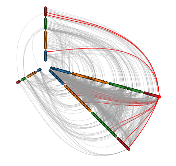
There are various layouts that you can choose from to visualize a network. All of the networks that you have seen so far have been drawn with a force-directed layout. However, one weakness that you may have noticed is that as the number of nodes and edges grows, the appearance of the graph looks more and more like a hairball such that there’s so much clutter that you can’t identify any meaningful patterns.

Academics are actively developing various types of layouts for large networks. One idea is to simply sample a subset of the network, but by doing so, you lose information. Another idea is to use a layout called a hive layout, which positions the nodes from the same class on linear axes and then draws the connections between them. You can read more about it here. By doing so, you’ll be able to find patterns that you wouldn’t if you were using a force layout. Below, I’ve taken a template from the D3.js website and adapted it to the petroleum trade network that we’ve seen in the previous posts:

Nodes of the same color belong to the same modularity class, which was calculated using gephi. You can see that similar nodes are grouped closer together and that the connections are denser between nodes of the same modularity class than they are between modularity classes. You can mouse over the nodes and edges to see which country each nodes represent and which countries each trade link connects. Each edge represents money flowing into a country. So United States -> Saudi Arabia means the US is importing petroleum.

For comparison, below is the same network, but drawn with a force-directed layout, which looks like a giant…hairball…sort of thing.

Here’s the code used to produce the json file:

R
1
2
3
4
5
6
7
8
9
10
11
12
13
14
15
16
17
18
19
20
21
22
23
24
25
26
27
28
29
30
31
32
33
34
35
36
37
38
39
40
41
42
43
44
45
46
47
48
49
50
51
52
53
54
55
56
57
58
59
60
61
62
63
64
65
66
67
68
69
70
71
72
73
74
75
76
77
78
library(sqldf)
 
#source urls for datafiles
trade_url <- "http://atlas.media.mit.edu/static/db/raw/year_origin_destination_hs07_6.tsv.bz2"
countries_url <- "http://atlas.media.mit.edu/static/db/raw/country_names.tsv.bz2"
 
#extract filenames from urls
trade_filename <- basename(trade_url)
countries_filename <- basename(countries_url)
 
#download data
download.file(trade_url,destfile=trade_filename)
download.file(countries_url,destfile=countries_filename)
 
#import data into R
trade <- read.table(file = trade_filename, sep = '\t', header = TRUE)
country_names <- read.table(file = countries_filename, sep = '\t', header = TRUE)
 
#extract petroleum trade activity from 2014
petro_data <- trade[trade$year==2014 & trade$hs07==270900,]
 
#we want just the exports to avoid double counting
petr_exp <- petro_data[petro_data$export_val != "NULL",]
 
#xxb doesn't seem to be a country, remove it
petr_exp <- petr_exp[petr_exp$origin != "xxb" & petr_exp$dest != "xxb",]
 
#convert export value to numeric
petr_exp$export_val <- as.numeric(petr_exp$export_val)
 
#take the log of the export value to use as edge weight
petr_exp$export_log <- log(petr_exp$export_val)
 
 
petr_exp$origin <- as.character(petr_exp$origin)
petr_exp$dest <- as.character(petr_exp$dest)
 
petr_exp <- sqldf("SELECT p.*, c.modularity_class as modularity_class_dest, d.modularity_class as modularity_class_orig, n.name as orig_name, o.name as dest_name
                   FROM petr_exp p
                   LEFT JOIN petr_class c
                    ON p.dest = c.id
                   LEFT JOIN petr_class d
                    ON p.origin = d.id
                   LEFT JOIN country_names n
                    ON p.origin = n.id_3char
                   LEFT JOIN country_names o
                    ON p.dest = o.id_3char")
petr_exp$orig_name <- gsub(" ","",petr_exp$orig_name, fixed=TRUE)
petr_exp$dest_name <-gsub(" ","",petr_exp$dest_name, fixed=TRUE)
petr_exp$orig_name <- gsub("'","",petr_exp$orig_name, fixed=TRUE)
petr_exp$dest_name <-gsub("'","",petr_exp$dest_name, fixed=TRUE)
 
petr_exp <- petr_exp[order(petr_exp$modularity_class_dest,petr_exp$dest_name),]
 
petr_exp$namestr_dest <- paste('Petro.Class',petr_exp$modularity_class_dest,'.',petr_exp$dest_name,sep="")
petr_exp$namestr_orig <- paste('Petro.Class',petr_exp$modularity_class_orig,'.',petr_exp$orig_name,sep="")
petr_names <- sort(unique(c(petr_exp$namestr_dest,petr_exp$namestr_orig)))
 
jsonstr <- '['
for(i in 1:length(petr_names)){
  curr_country <- petr_exp[petr_exp$namestr_dest==petr_names[i],]
  jsonstr <- paste(jsonstr,'\n{"name":"',petr_names[i],'","size":1000,"imports":[',sep="")
  if(nrow(curr_country)==0){
    jsonstr <- jsonstr
  } else {
      for(j in 1:nrow(curr_country)){
        jsonstr <- paste(jsonstr,'"',curr_country$namestr_orig[j],'"',sep="")
        if(j != nrow(curr_country)){jsonstr <- paste(jsonstr,',',sep="")}
      }
  }
  jsonstr <- paste(jsonstr,']}',sep="")
  if(i != length(petr_names)){jsonstr <- paste(jsonstr,',',sep="")}
}
jsonstr <- paste(jsonstr,'\n]',sep="")
 
fileConn <- file("exp_hive.json")
writeLines(jsonstr, fileConn)
close(fileConn)

Posted in: Mathematics

No. 123: 25 Days of Network Theory – Day 6 – Relative Importance of Ex-Soviet Countries in the Petroleum Trade

10 July, 2017 10:58 PM / 1 Comment / Gene Dan

I had originally intended to create graphics for all the world’s countries, but the resulting visualizations looked so cluttered that I felt like I was tripping on acid, so I reduced the scope of today’s post to those nations that used to belong to the Soviet Union.

From the original intention of the post, I changed the petroleum dataset to draw from an MIT dataset going all the way back to 1962, although in retrospect that was unnecessary. A friend of mine suggested that I create some kind of visualization that varied over time, so I’ve done just that. I used igraph to create a network for each year, calculated the eigenvector centrality of each node for each network, and then calculated the relative importance of the ex-Soviet countries to each other in the international sphere.

You can see from these visualizations that immediately after the breakup, Russia was the dominant player, but as the years have gone by, other countries like Azerbaijan and Kazakhstan have become increasingly important, and for this particular commodity, Russia’s power is declining:

Selection_282

I felt like these templates weren’t designed to handle all the ex-Soviet countries, so for the top visualization I hand picked 4 countries that I believed had the most influence. Here’s all of them together:

R
1
2
3
4
5
6
7
8
9
10
11
12
13
14
15
16
17
18
19
20
21
22
23
24
25
26
27
28
29
30
31
32
33
34
35
36
37
38
39
40
41
42
43
44
45
46
47
48
49
50
51
52
53
54
55
56
57
58
59
60
61
62
63
64
65
66
67
68
69
70
71
72
73
74
75
76
77
78
79
80
81
82
83
84
85
86
87
88
89
90
91
92
93
94
95
96
97
98
99
100
101
102
103
104
105
106
107
108
109
110
111
112
113
114
115
116
117
118
119
120
121
122
123
library(sqldf)
library(rgexf)
library(igraph)
library(reshape2)
library(plyr)
 
#source urls for datafiles
trade_url <- "http://atlas.media.mit.edu/static/db/raw/year_origin_destination_sitc_rev2.tsv.bz2"
countries_url <- "http://atlas.media.mit.edu/static/db/raw/country_names.tsv.bz2"
 
#extract filenames from urls
trade_filename <- basename(trade_url)
countries_filename <- basename(countries_url)
 
#download data
download.file(trade_url,destfile=trade_filename)
download.file(countries_url,destfile=countries_filename)
 
#import data into R
trade <- read.table(file = trade_filename, sep = '\t', header = TRUE)
country_names <- read.table(file = countries_filename, sep = '\t', header = TRUE)
 
 
#extract petroleum trade activity
petro_data <- trade[trade$sitc==3330,]
 
#we want just the exports to avoid double counting
petr_exp <- petro_data[petro_data$export_val != "0.00",]
 
#xxb doesn't seem to be a country, remove it
petr_exp <- petr_exp[!(petr_exp$origin %in% c("xxa","xxb","xxc","xxd","xxe","xxf","xxg", "xxh")) & !(petr_exp$dest %in% c("xxa","xxb","xxc","xxd","xxe","xxf","xxg", "xxh")),]
 
#convert export value to numeric
petr_exp$export_val <- as.numeric(petr_exp$export_val)
 
petr_exp$origin <- as.character(petr_exp$origin)
petr_exp$dest <- as.character(petr_exp$dest)
 
 
#take the log of the export value to use as edge weight
petr_exp$export_log <- log(petr_exp$export_val)
 
 
#generate a data frame with eigenvector centrality for each year
#there is a separate network generated for each year
petro_eigendata <- c()
 
for(j in 1992:2014){
#for(j in 2000:2014){  
petr_exp_curryear <- petr_exp[petr_exp$year==j,]
 
 
#build edges
petr_exp_curryear$edgenum <- 1:nrow(petr_exp_curryear)
petr_exp_curryear$edges <- paste('<edge id="', as.character(petr_exp_curryear$edgenum),'" source="', petr_exp_curryear$dest, '" target="',petr_exp_curryear$origin, '" weight="',petr_exp_curryear$export_log,'"/>',sep="")
 
 
#build nodes
nodes <- data.frame(id=sort(unique(c(petr_exp_curryear$origin,petr_exp_curryear$dest))))
nodes <- sqldf("SELECT n.id, c.name
               FROM nodes n
               LEFT JOIN country_names c
               ON n.id = c.id_3char")
 
nodes$nodestr <- paste('<node id="', as.character(nodes$id), '" label="',nodes$name, '"/>',sep="")
 
#build metadata
gexfstr <- '<?xml version="1.0" encoding="UTF-8"?>
<gexf xmlns:viz="http:///www.gexf.net/1.1draft/viz" version="1.1" xmlns="http://www.gexf.net/1.1draft">
<meta lastmodifieddate="2010-03-03+23:44">
<creator>Gephi 0.7</creator>
</meta>
<graph defaultedgetype="undirected" idtype="string" type="static">'
 
#append nodes
gexfstr <- paste(gexfstr,'\n','<nodes count="',as.character(nrow(nodes)),'">\n',sep="")
fileConn<-file("exp_curryear.gexf")
for(i in 1:nrow(nodes)){
  gexfstr <- paste(gexfstr,nodes$nodestr[i],"\n",sep="")}
gexfstr <- paste(gexfstr,'</nodes>\n','<edges count="',as.character(nrow(petr_exp_curryear)),'">\n',sep="")
 
#append edges and print to file
for(i in 1:nrow(petr_exp_curryear)){
  gexfstr <- paste(gexfstr,petr_exp_curryear$edges[i],"\n",sep="")}
gexfstr <- paste(gexfstr,'</edges>\n</graph>\n</gexf>',sep="")
writeLines(gexfstr, fileConn)
close(fileConn)
 
#Import gexf file and convert to igraph object
petr_exp_curryear_gexf <- read.gexf("exp_curryear.gexf")
petr_exp_curryear_igraph <- gexf.to.igraph(petr_exp_curryear_gexf)
 
curryear_eigen_centrality <- eigen_centrality(petr_exp_curryear_igraph,directed=TRUE,weight=edge_attr(petr_exp_curryear_igraph)$weight)$vector
 
curryear_eigendata <- data.frame(date=j,curryear_eigen_centrality)
curryear_eigendata$country <- rownames(curryear_eigendata)
rownames(curryear_eigendata) <- NULL
 
#curryear_eigendata <- curryear_eigendata[curryear_eigendata$country %in% c("United States","Netherlands","United Kingdom","China","Russia"),]
curryear_eigendata <- curryear_eigendata[curryear_eigendata$country %in% c("Russia","Ukraine","Armenia","Azerbaijan","Belarus","Estonia","Georgia","Kazakhstan","Kyrgyzstan","Latvia","Lithuania","Moldova","Tajikistan","Turkmenistan","Uzbekistan"),]
#curryear_eigendata <- curryear_eigendata[order(-curryear_eigen_centrality),]
#curryear_eigendata <- curryear_eigendata[c(1:4),]
 
curryear_eigendata$eigen_pct <- (curryear_eigendata$curryear_eigen_centrality/sum(curryear_eigendata$curryear_eigen_centrality)) * 100
 
curryear_eigen_pct <-dcast(curryear_eigendata,date~country,value.var="eigen_pct")
 
 
petro_eigendata <- rbind.fill(petro_eigendata,curryear_eigen_pct)
}
 
petro_eigendata[is.na(petro_eigendata)] <- 0
 
#export for stack diagram
write.table(petro_eigendata,file='petro_eigendata.tsv',quote=FALSE,sep='\t',row.names=FALSE)
 
#export for show reel
petro_long <- melt(petro_eigendata,id.vars="date")
names(petro_long) <- c("date","symbol","price")
petro_long <- petro_long[petro_long$symbol %in% c("Russia","Kazakhstan","Ukraine","Azerbaijan"),]
petro_long$symbol <- ifelse(petro_long$symbol=="Russia","RUS",ifelse(petro_long$symbol=="Kazakhstan","KAZ",ifelse(petro_long$symbol=="Ukraine","UKR","AZE")))
 
write.csv(petro_long,file='petro_long.csv',quote=FALSE,row.names=FALSE)

Posted in: Mathematics

Post Navigation

« Previous 1 2 3 4 … 10 Next »

Archives

  • September 2023
  • February 2023
  • January 2023
  • October 2022
  • March 2022
  • February 2022
  • December 2021
  • July 2020
  • June 2020
  • May 2020
  • May 2019
  • April 2019
  • November 2018
  • September 2018
  • August 2018
  • December 2017
  • July 2017
  • March 2017
  • November 2016
  • December 2014
  • November 2014
  • October 2014
  • August 2014
  • July 2014
  • June 2014
  • February 2014
  • December 2013
  • October 2013
  • August 2013
  • July 2013
  • June 2013
  • March 2013
  • January 2013
  • November 2012
  • October 2012
  • September 2012
  • August 2012
  • July 2012
  • June 2012
  • May 2012
  • April 2012
  • March 2012
  • February 2012
  • January 2012
  • December 2011
  • September 2011
  • August 2011
  • July 2011
  • June 2011
  • January 2011
  • December 2010
  • October 2010
  • September 2010
  • August 2010
  • June 2010
  • May 2010
  • April 2010
  • March 2010
  • September 2009
  • August 2009
  • May 2009
  • December 2008

Categories

  • Actuarial
  • Cycling
  • Logs
  • Mathematics
  • MIES
  • Music
  • Uncategorized

Links

Cyclingnews
Jason Lee
Knitted Together
Megan Turley
Shama Cycles
Shama Cycles Blog
South Central Collegiate Cycling Conference
Texas Bicycle Racing Association
Texbiker.net
Tiffany Chan
USA Cycling
VeloNews

Texas Cycling

Cameron Lindsay
Jacob Dodson
Ken Day
Texas Cycling
Texas Cycling Blog
Whitney Schultz
© Copyright 2025 - Gene Dan's Blog
Infinity Theme by DesignCoral / WordPress