• Home
  • Readings
  • Github
  • MIES
  • TmVal
  • About
Gene Dan's Blog

Category Archives: Mathematics

No. 116: 70 Days of Linear Algebra (Day 9)

30 November, 2016 6:51 PM / Leave a Comment / Gene Dan

Section: 1.6 – Applications of Linear Systems

Linear systems can be used to model and solve problems concerning traffic flow. Consider for instance, the following set of intersections modeled by a graph:

selection_338

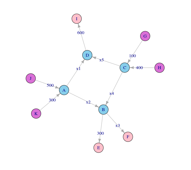
The orchid nodes G, H, J, and K represent traffic inflows. The pink nodes E, F, and I represent traffic outflows. The blue nodes A, B, C, and D represent intersections. Each edge (the lines connecting the nodes – representing roads) is labeled with the traffic flow measured in cars per hour. For example, 500 cars travel from J to A each hour. Assuming that for each intersection (and for the network as a whole), that traffic inflow equals traffic outflow, one question arises regarding capacity – how much traffic should the roads x1, x2, x3, x4, and x5 be designed to handle?

First, we need to determine traffic inflows and outflows for each intersection:

Intersection Flow In Flow Out
A 300 + 500 x1 + x2
B x2 + x4 300 + x3
C 400 + 100 x4 + x5
D x1 + x5 600

In addition, we have the constraint that total network inflow (500 + 300 + 100 + 400) equal total network outflow (300 + x3 + 600), so x3 = 400.

We can use this information to represent the network as a system of linear equations and row reduce the corresponding augmented matrix to solve for the unknowns:

\[\begin{aligned} x_1+x_2&=800\\x_2-x_3+x_4&=300\\x_4+x_5&=500\\x_1+x_5&=600\\x_3&=400\end{aligned}\]

\[\left[\begin{array}{cccccc} 1 & 1 & 0 & 0 & 0 & 800 \\ 0 & 1 & -1 & 1 & 0 & 300 \\ 0 & 0 & 0 & 1 & 1 & 500 \\ 1 & 0 & 0 & 0 & 1 & 600 \\ 0 & 0 & 1 & 0 & 0 & 400 \\ \end{array}\right] \sim \left[\begin{array}{cccccc} 1 & 0 & 0 & 0 & 1 & 600 \\ 0 & 1 & 0 & 0 & -1 & 200 \\ 0 & 0 & 1 & 0 & 0 & 400 \\ 0 & 0 & 0 & 1 & 1 & 500 \\ 0 & 0 & 0 & 0 & 0 & 0 \end{array} \right] \]

Which leads us to the general solution:

\[\left\{\begin{aligned} x_1 & = 600 – x_5 \\ x_2 &=200+x_5 \\ x_3&=400\\x_4&=500-x_5\\x_5&\text{ is free} \end{aligned}\right.\]

Since x5 is free, we have infinitely many solutions to the problem. Thus, in practice, how we actually design the roads would depend on how much traffic we anticipate for x5.

Code used to create the graph

R
1
2
3
4
5
6
7
8
9
10
11
12
13
14
15
16
17
18
19
20
21
22
23
24
25
26
27
28
29
30
31
32
33
34
35
36
37
38
39
40
41
42
43
library(igraph)
 
edges <- c("B","E"
          ,"B","F"
          ,"A","B"
          ,"C","B"
          ,"G","C"
          ,"H","C"
          ,"C","D"
          ,"D","I"
          ,"J","A"
          ,"K","A"
          ,"A","D")
 
edge_labels <- c("300"
                ,"x3"
                ,"x2"
                ,"x4"
                ,"100"
                ,"400"
                ,"x5"
                ,"600"
                ,"500"
                ,"300"
                ,"x1")
 
cols <- c("skyblue"
          ,"pink"
          ,"pink"
          ,"skyblue"
          ,"skyblue"
          ,"orchid"
          ,"orchid"
          ,"skyblue"
          ,"pink"
          ,"orchid"
          ,"orchid")
traffic <- graph(x) %>% set_edge_attr("label",value=edge_labels)
traffic$label <- edge_labels
plot(traffic
    ,vertex.color=cols
    ,edge.arrow.size=.4
)

Code used to solve the equations

R
1
2
3
4
5
6
7
8
library(pracma)
A = matrix(c(1,1,0,0,0,800
            ,0,1,-1,1,0,300
            ,0,0,0,1,1,500
            ,1,0,0,0,1,600
            ,0,0,1,0,0,400)
            ,nrow=5,ncol=6,byrow=TRUE)
rref(A)

Posted in: Mathematics / Tagged: 70 days of linear algebra

No. 115: The Collatz Conjecture

22 November, 2016 7:52 PM / Leave a Comment / Gene Dan

The Collatz Conjecture is a famous unsolved problem in mathematics. Given any positive integer, if that integer is even, divide it by two. If it’s odd, multiply it by three and then add 1. Keep repeating until you get 1. The conjecture claims that no matter what number you start with, you will always reach 1.

Is this the case? Nobody knows! But let’s try a few examples: 12, 7, and 9

12 -> 6 -> 3 -> 10 -> 5 -> 16 -> 8 -> 4 -> 2 -> 1
7 -> 22 -> 11 -> 34 -> 17 -> 52 -> 26 -> 13 -> 40 -> 20 -> 10 -> 5 -> 16 -> 8 -> 4 -> 2 -> 1
9 -> 28 -> 14 -> 7 -> … 8 -> 4 -> 2 -> 1

In all three cases, we get a chain of numbers that eventually leads to 1. In fact, we can try every integer up to 100 million and we will still end up with 1! Given that a counterexample hasn’t been found for extremely large numbers, many people believe the conjecture to be true. The reason why this problem is so famous is because it’s easy to understand, but hard to solve.

Given the example above, we can construct a directed graph that plots each successive step for all situations up to a specified integer. For example, when n = 50:

selection_088

We can see that every chain leads to 1, which is why so many arrows point to node 1. I’ve created a visualization using R Shiny, and using the slider below, you can see how the graph changes as you change n. I could go on about R Shiny, which is an extremely useful package for visualizing mathematical concepts due to its interactive nature, but since I’m busy, I’ll have to save that for a later time.

The code is contained in 3 files, server.R, ui.r, and helpers.R.

server.R:

R
1
2
3
4
5
6
7
8
9
10
11
12
13
14
15
16
17
18
19
20
21
22
23
24
25
26
27
28
29
30
31
library(shiny)
library(igraph)
source("helpers.R")
shinyServer(function(input, output) {
  
  output$distPlot <- renderPlot({
    out.n <- input$n
    pairs <- c()
    for(i in 1:out.n)
    {
      curr <- i
      while(curr != 1)
      {
        if(curr %% 2 == 0)
        {
          nxt <- curr / 2
        }
        else
        {
          nxt <- 3 * curr + 1
        }
        pairs <- c(pairs,as.character(curr),as.character(nxt))
        curr <- nxt
      }
    }
    graph.directed <- graph(pairs)
    l <- layout.forceatlas2(graph.directed, iterations=100,plotstep=0)
    plot(graph.directed,layout=l, vertex.color="skyblue", vertex.size=6, edge.arrow.size=.2, vertex.label.cex=.5)
  })
  
})

ui.r

1
2
3
4
5
6
7
8
9
10
11
12
13
14
15
16
17
18
19
20
21
22
23
24
25
26
27
28
29
30
31
32
33
34
35
36
37
38
39
40
41
42
43
44
45
library(shiny)
 
shinyUI(fluidPage(
  
  # Application title
  titlePanel("Collatz Conjecture"),
  withMathJax(
  HTML("Consider the following operation on an arbitrary positive integer:
            <ul>
            <li>If the number is even, divide it by two.</li>
            <li>If the number is odd, triple it and add one.</li>
            </ul></br>
  In modular arithmetic notation, define the function \\(f\\) as follows:</br>
$$f(x)= \\left\\{
\\begin{aligned}
     \\ n/2  &\\quad  \\text{if } n\\equiv0\\,(\\text{mod } 2)  \\\\
     \\ 3n+1 &\\quad  \\text{if } n\\equiv1\\,(\\text{mod } 2)  \\\\
     \\end{aligned}
     \\right.$$
  Now, form a sequence by performing this operation repeatedly, beginning with any positive integer, and taking the result at each step as the input at the next.
       In notation:
$$a_i=\\left\\{
       \\begin{aligned}
       \\ n          & \\quad \\text{for } i = 0 \\\\
       \\ f(a_{i-1}) & \\quad \\text{for i} >0 \\\\
       \\end{aligned}
       \\right.$$
  The Collatz conjecture is: <i>This process will eventually reach the number 1, regardless of which positive integer is chosen initially</i>.")),
  
  # Sidebar with a slider input for K
  sidebarLayout(
    sidebarPanel(
       sliderInput("n",
                   "Directed graph for all sequences up to n:",
                   min = 2,
                   max = 100,
                   value = 50)
    ),
    
    
    mainPanel(
       plotOutput("distPlot",width="500px", height="500px")
    )
  )
))

The helpers.R file was taken here, and was used to apply the ForceAtlas 2 layout on the igraph package.

Posted in: Mathematics

No. 114: Visualizing the Blockchain

24 December, 2014 5:29 PM / Leave a Comment / Gene Dan

For those of you who don’t know what Bitcoin is, it’s a digital currency that’s been gaining attention over the last few years, mostly due to its obscure user base, popularity on the black market (although most bitcoin transactions are legal), and its exchange rate volatility versus the U.S. dollar.

I’ve been interested in Bitcoin for quite some time, since unlike cash transactions, all bitcoin transactions are recorded on a publicly available ledger called the Blockchain. Because the blockchain records all transactions that occur over the bitcoin network, it can be a valuable source of information, revealing interesting patterns about peer-to-peer monetary transactions that were previously unavailable under traditional currency, due to lack of available data.

I stumbled across some CSV files on the internet that contain parsed blockchain information available in a script-friendly format here. Using this dataset I wrote a script to extract the transactions from the first 500 bitcoin users:

1
2
3
4
5
6
7
8
9
10
11
12
13
14
15
16
17
18
19
20
21
22
23
24
25
26
27
28
29
30
31
32
33
34
35
36
37
38
39
40
#import dataset
#edges <- read.csv("user_edges.txt", header=FALSE)
#head(edges)
 
###subset first n users
lim <- 500
edges.sub <- edges[edges$V2 <= lim & edges $V3 <= lim & (edges$V2 != edges$V3), c("V2","V3")]
head(edges.sub,500)
sub.unique <- edges.sub[!duplicated(edges.sub),]
sub.unique$edgenum <- 1:nrow(sub.unique)
head(sub.unique)
sub.unique$edges <- paste('<edge id="', as.character(sub.unique$edgenum),'" source="', sub.unique$V2, '" target="',sub.unique$V3, '"/>',sep="")
 
###build nodes
nodes <- data.frame(id=sort(unique(c(sub.unique$V2,sub.unique$V3))))
nodes$nodestr <- paste('<node id="', as.character(nodes$id), '" label="',nodes$id, '"/>',sep="")
head(nodes)
 
### build metadata
gexfstr <- '<?xml version="1.0" encoding="UTF-8"?>
<gexf xmlns:viz="http:///www.gexf.net/1.1draft/viz" version="1.1" xmlns="http://www.gexf.net/1.1draft">
<meta lastmodifieddate="2010-03-03+23:44">
<creator>Gephi 0.7</creator>
</meta>
<graph defaultedgetype="undirected" idtype="string" type="static">'
 
 
### append nodes
gexfstr <- paste(gexfstr,'\n','<nodes count="',as.character(nrow(nodes)),'">\n',sep="")
fileConn<-file("output.gexf")
for(i in 1:nrow(nodes)){
  gexfstr <- paste(gexfstr,nodes$nodestr[i],"\n",sep="")}
gexfstr <- paste(gexfstr,'</nodes>\n','<edges count="',as.character(nrow(sub.unique)),'">\n',sep="")
 
### append edges and print to file
for(i in 1:nrow(sub.unique)){
  gexfstr <- paste(gexfstr,sub.unique$edges[i],"\n",sep="")}
gexfstr <- paste(gexfstr,'</edges>\n</graph>\n</gexf>',sep="")
writeLines(gexfstr, fileConn)
close(fileConn)

I subsequently imported the output file into gephi to create a network visualization of the transactions. You can view the process in the video below.

https://www.youtube.com/watch?v=wjw0ksaRSO4&feature=youtu.be

The resulting graph:

Transactions amongst the first 500 users of Bitcoin

Transactions amongst the first 500 users of Bitcoin

Here you can see that the modularity algorithms have identified clusters of tightly-knit users who transact frequently with each other, along with influential users who may be running businesses or may be serving as middlemen between other groups of users.

Posted in: Logs, Mathematics / Tagged: bitcoin, blockchain, graph, network

No. 113: International Flight Paths

30 November, 2014 7:48 PM / 1 Comment / Gene Dan

So asĀ  continuation from my last post, I’ve decided to map out all the major air traffic routes worldwide. Data were obtained from openflights, with the individual airport data here and the route data here. You can see the processed gexf file here. I’ve started work on creating an automated script to convert raw data into a .gexf file. It’s not quite done yet, but the script used to do so can be found below:

1
2
3
4
5
6
7
8
9
10
11
12
13
14
15
16
17
18
19
20
21
22
23
24
25
26
27
28
29
30
31
32
33
34
35
setwd("./openflights-code-769/openflights/data")
 
### create node XML
airports <- read.csv("airports.dat",header=FALSE)
head(airports)
airports$nodes <- paste('<node id="', as.character(airports$V1), '.0" label="',airports$V5, '"/>',sep="")
 
### create edge XML
routes <- read.csv("routes.dat",header=FALSE)
routes$edgenum <- 1:nrow(routes)
head(routes)
routes$edges <- paste('<edge id="', as.character(routes$edgenum),'.0" source="', routes$V3, '" target="',routes$V5, '"/>',sep="")
 
### build metadata
gexfstr <- '<?xml version="1.0" encoding="UTF-8"?>
<gexf xmlns:viz="http:///www.gexf.net/1.1draft/viz" version="1.1" xmlns="http://www.gexf.net/1.1draft">
<meta lastmodifieddate="2010-03-03+23:44">
<creator>Gephi 0.7</creator>
</meta>
<graph defaultedgetype="undirected" idtype="string" type="static">'
 
### append nodes
gexfstr <- paste(gexfstr,'\n','<nodes count="',as.character(nrow(airports)),'">\n',sep="")
fileConn<-file("output.gexf")
for(i in 1:nrow(airports)){
gexfstr <- paste(gexfstr,airports$nodes[i],"\n",sep="")}
gexfstr <- paste(gexfstr,'</nodes>\n','<edges count="',as.character(nrow(routes)),'">\n',sep="")
 
 
### append edges and print to file
for(i in 1:nrow(routes)){
  gexfstr <- paste(gexfstr,routes$edges[i],"\n",sep="")}
gexfstr <- paste(gexfstr,'</edges>\n</graph>\n</gexf>',sep="")
writeLines(gexfstr, fileConn)
close(fileConn)

I’ve created three separate graphs using different measures of influence – Betweenness Centrality, Eigenvector Centrality, and Degree. Click on an image to expand the graph, although be aware that it may take a while to load.

Selection_001

Node and text size based on betweenness centrality

You’ll notice that some airports such as LAX, which weren’t noteworthy in the graphs depicting domestic flight routes have gained new prominence from an international perspective since they serve as important traffic hubs for overseas flights. Other important airports include Dubai International Airport (DXB), Beijing Capital International Airport (PEK), Charles De Gaulle International Airport (CDG), and interestingly, Anchorage International Airport (ANC).

Selection_002

Node and text size based on eigenvector centrality

Selection_003

Node and text size based on degree

Posted in: Mathematics / Tagged: international flight network graph, international flight routes

No. 112: Flight Routes in the United States

22 November, 2014 4:30 PM / Leave a Comment / Gene Dan

Check out these network graphs I made that show domestic flight routes in the United States. You can take a look at the data set here. The following network diagram displays airports as nodes (the circles in the graph) and routes between airports as edges (the lines between the circles). The size of the circles is based on a measure called betweenness centrality, which is a measure of an airport’s influence within the network.

air2

Node size based on betweenness centrality

So, there are a couple of things that stand out – first, even without any information dealing with the number of passengers, betweenness centrality has identified some of the busiest airports in the United States. Second, when I created the input dataset, I stripped the file of all geographic information. Even so, if you invert the graph and rotate it a little you might be able to get an image that closely matches the geographic locations of the airports.

The two tails represent airports from remote parts of the United States – Alaska and Guam.

Below is another diagram, with the difference that node size is calculated via eigenvector centrality rather than betweenness centrality. With respect to eigenvector centrality, nodes are given a higher score if they are connected to other nodes that have a high score, and less otherwise.

Node size based on eigenvector centrality

Node size based on eigenvector centrality

Posted in: Mathematics, Uncategorized / Tagged: domestic air traffic, domestic flight paths, graph theory, network diagram, US flight paths

Post Navigation

« Previous 1 2 3 4 5 6 … 10 Next »

Archives

  • September 2023
  • February 2023
  • January 2023
  • October 2022
  • March 2022
  • February 2022
  • December 2021
  • July 2020
  • June 2020
  • May 2020
  • May 2019
  • April 2019
  • November 2018
  • September 2018
  • August 2018
  • December 2017
  • July 2017
  • March 2017
  • November 2016
  • December 2014
  • November 2014
  • October 2014
  • August 2014
  • July 2014
  • June 2014
  • February 2014
  • December 2013
  • October 2013
  • August 2013
  • July 2013
  • June 2013
  • March 2013
  • January 2013
  • November 2012
  • October 2012
  • September 2012
  • August 2012
  • July 2012
  • June 2012
  • May 2012
  • April 2012
  • March 2012
  • February 2012
  • January 2012
  • December 2011
  • September 2011
  • August 2011
  • July 2011
  • June 2011
  • January 2011
  • December 2010
  • October 2010
  • September 2010
  • August 2010
  • June 2010
  • May 2010
  • April 2010
  • March 2010
  • September 2009
  • August 2009
  • May 2009
  • December 2008

Categories

  • Actuarial
  • Cycling
  • Logs
  • Mathematics
  • MIES
  • Music
  • Uncategorized

Links

Cyclingnews
Jason Lee
Knitted Together
Megan Turley
Shama Cycles
Shama Cycles Blog
South Central Collegiate Cycling Conference
Texas Bicycle Racing Association
Texbiker.net
Tiffany Chan
USA Cycling
VeloNews

Texas Cycling

Cameron Lindsay
Jacob Dodson
Ken Day
Texas Cycling
Texas Cycling Blog
Whitney Schultz
© Copyright 2025 - Gene Dan's Blog
Infinity Theme by DesignCoral / WordPress