Category Archives: Mathematics

No. 99: Eratosthenes’ Sieve

26 August, 2013 8:29 PM / Leave a Comment / Gene Dan

A friend of mine pointed out that I had skipped a few steps in the solution I posted yesterday for Euler #3 – first, I didn’t actually go through the process of finding the primes, and second, I didn’t try to figure out how many prime numbers would be necessary for the list I used to find the largest prime factor of 600,851,475,143. To rectify these issues, I wrote another program that can provide the general solution for any integer larger than 1:

prime <- 2
primes <-c()
remaining.factor <- 600851475143
while(prime != remaining.factor){
  while(remaining.factor %% prime ==0){
    remaining.factor <- remaining.factor/prime
  }
  primes <- append(primes,prime)
  while(length(which(prime %% primes ==0)>0)){
    prime <- prime + 1
  }
}
remaining.factor

prime <- 2

primes <-c()

remaining.factor <- 600851475143

while(prime != remaining.factor){

while(remaining.factor %% prime ==0){

remaining.factor <- remaining.factor/prime

}

primes <- append(primes,prime)

while(length(which(prime %% primes ==0)>0)){

prime <- prime + 1

}

remaining.factor

All you have to do is replace 600,851,475,143 with a number of your choice, and the script above will find the largest prime factor for that number, given enough time and memory. I was actually somewhat lucky that the answer ended up being 6857. Had it been larger, the program might have taken much longer to execute (possibly impractically long if the factor happened to be big enough).

Eratosthenes’ Sieve

Now that I have that out of the way, I would like to demonstrate a method for quickly generating prime numbers, called Eratosthenes’ Sieve. You can embed this algorithm into the solution of any Project Euler problem that calls for a large list of prime numbers under 10 million (after 10 million, the algorithm takes a long time to execute, and other sieves may be a better choice). While it’s possible to generate prime numbers on the fly for Euler problems, I still prefer to use lists to solve them. Below is the algorithm for Eratosthenes’ Sieve that I’ve written in R:

primes <- 2:10000000

curr.prime <- 2
while(curr.prime < sqrt(10000000)){
  primes[(primes >= curr.prime **2) & (primes %% curr.prime == 0)] <- 0
  curr.prime <- min(primes[primes>curr.prime])
}

primes <- primes[primes!=0]

primes <- 2:10000000

curr.prime <- 2

while(curr.prime < sqrt(10000000)){

primes[(primes >= curr.prime **2) & (primes %% curr.prime == 0)] <- 0

curr.prime <- min(primes[primes>curr.prime])

}

primes <- primes[primes!=0]

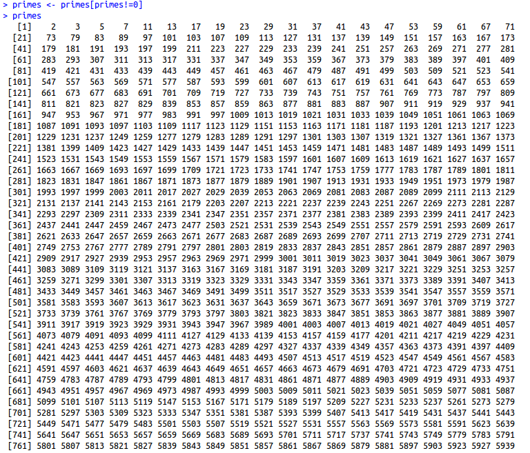
The script above will generate a list of all the primes below 10,000,000. The algorithm starts with a list of integers from 2 to 10,000,000. Starting with 2, the smallest prime, you remove all the multiples of 2 from the list. Then you move on to the next prime, 3, and remove all the multiples of 3 from the list. The process continues until the only numbers left in the list are prime numbers.

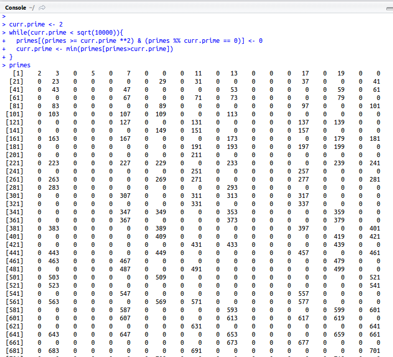
As you can see, all the composite numbers are now marked as zeros. The final line of the script removes these zeros and gives you a list of just the prime numbers.

Posted in: Mathematics / Tagged: eratosthenes sieve, eratosthenes sieve in r, project euler 3, project euler 3 r, R

No. 98: Project Euler #3 – Largest Prime Factor (solution in R)

25 August, 2013 1:15 PM / 1 Comment / Gene Dan

Question:

The prime factors of 13195 are 5, 7, 13 and 29.
What is the largest prime factor of the number 600851475143 ?

Approach:

Every integer greater than one has a unique prime factorization. This means that each integer greater than one can be represented as a unique product of prime numbers. For example, the number 5,784 can be written as:

\[2^3\times 241\]

Where 2 and 241 are prime. Likewise, the number 54,887,224 can be written as:

\[2^3\times 7 \times 53 \times 18493\]

Where 2, 7, 53, and 18493 are prime. For this problem, our goal is to find the largest prime factor of the number 600,851,475,143. An interesting thing to note is that the mathematician F. N. Cole, back in 1903, found the prime factorization of the number 147,573,952,589,676,412,927, which is 193,707,721 × 761,838,257,287. It took him three years worth of effort to do so. While our number is not quite as large as Cole’s, such problems today are trivial. Computer algebra systems such as Mathematica can factorize large numbers very quickly. What took Cole 3 years back in 1903 now takes less than a second today.

We have some discretion in our approach to solving this problem. You can probably use Mathematica to solve it with a single line of code. On the other hand, if you’re using a bare programming language like C++, you would probably need to write more code. Your choice on what to do depends on what you want to learn from solving the problem. I had previously solved this problem using VBA which first involved creating a list of prime numbers, using the list to find the prime factors of 600,851,475,143, and then selecting the largest one as my answer. With R, I’ve taken a middle approach, compromising between arriving at an immediate answer with a computer algebra system and having to create a list of primes from scratch. In this case, I used a list of primes I found off a website and saved them into a file called primes.csv. My mental outline is as follows:

1. Obtain a list of prime numbers
2. Find which of these prime numbers divide 600,851,475,143 evenly.
3. Of the primes that divide 600,851,475,143 evenly, find the largest one.

Solution:

primes <- sort(as.vector(as.matrix(read.csv("primes.csv",header=FALSE))))
max(primes[which(600851475143 %% primes == 0)])

1 2	primes <- sort(as.vector(as.matrix(read.csv("primes.csv",header=FALSE)))) max(primes[which(600851475143 %% primes == 0)])

The first line does five things. First, it imports the list of prime numbers as a data frame, then converts the data frame into a matrix, then converts the matrix into a vector, and then sorts the primes within the vector in ascending order. This vector is then assigned to the variable primes. The second line accomplishes three things. The which() function returns the indices of the elements that divide 600,851,475,143 evenly. These indices are then used to extract the corresponding elements of the vector primes. Finally, the function max() returns the largest of these primes, giving us the answer, 6857.

I thought this answer would avoid the tedium of having to calculate each prime myself, but was not so trivial that I could find the answer without learning anything. I thought this method was a good way to demonstrate the use of indexing to find the solution.

Posted in: Mathematics / Tagged: largest prime factor, prime factorization, project euler, project euler 3, project euler 3 r, solution in r

No. 97: Project Euler #2 – Even Fibonacci Numbers

19 August, 2013 6:54 PM / Leave a Comment / Gene Dan

Question:

Each new term in the Fibonacci sequence is generated by adding the previous two terms. By starting with 1 and 2, the first 10 terms will be:
1, 2, 3, 5, 8, 13, 21, 34, 55, 89, …
By considering the terms in the Fibonacci sequence whose values do not exceed four million, find the sum of the even-valued terms.

Background:

There are some interesting things to note about Fibonnaci. Students often get their first introduction to the Fibonacci numbers when they first learn about sequences. The popular story is that they were used by Fibonacci to model rabbit populations over a period of time – you start with one pair of rabbits, denoted by 1 as the first term of the sequence. After a month, this pair of rabbits produces another pair, and now the total number of pairs is two. After another month, these two pairs produce another pair, resulting in a total of three pairs after two months. After three months, these three pairs produce 2 additional pairs, resulting in a total of five. The sequence then continues indefinitely, and students are often surprised at how quickly the terms grow.

Beyond the Fibonnaci numbers, there are some more interesting things about the mathematician for whom they are named, and how he fits in with the history of mathematics. While the Fibonacci numbers may be the most widespread way in which people are aware of Fibonacci’s existence, they are not (at least in my opinion), his most important contribution to western mathematics. Although the Fibonacci numbers appear in his book, Liber Abaci, the book itself also introduces the Hindu-Arabic number system, and it was this book that played a crucial role in popularizing the Arabic numerals – the numbers we use today – in western society. Prior to that, Europeans relied on Roman Numerals, which were cumbersome when it came to calculation. Even though the Arabic numerals appeared in Liber Abaci in 1202, it took another 400 years until they became ubiquitous throughout Europe, when the invention of the printing press aided in its widespread adoption.

Approach:

This problem is fairly straightforward. The description already tells you how to calculate the Fibonnaci numbers, and simply asks you to find the sum of the even valued terms which are less than four million. With some time and effort, you could easily do the problem by hand, although there is more educational value beyond simple addition (and efficiency!) if you solve it with a computer program. When I start out on these problems, I first create a mental outline of the solution, typically starting with brute force, and if I realize that a brute force solution would take too long, I try to come up with an indirect approach that may be more efficient. In this case the problem is simple, so I decided to use brute force. Here are steps in my mental outline:

Generate the sequence of all Fibonacci numbers that are less than 4,000,000.
Determine which numbers of the sequence are even numbers, then extract this subset.
Add the subset of these even numbers. This will be the solution.

Solution 1:

x <- c(1,2)
k = 3
i = 3
while(k<=4000000){
  x <- append(x,k)
  k = k + x[i-1]
  i = i +1
}
sum(x[x%%2==0])

x <- c(1,2)

k = 3

i = 3

while(k<=4000000){

x <- append(x,k)

k = k + x[i-1]

i = i +1

}

sum(x[x%%2==0])

For this solution, I first created a vector x containing the first two seed values, 1 and 2. This vector will be used to store the sequence of Fibonnaci numbers under 4 million. Next, I declared variables k and i, starting at 3 to be used as indices in the while loop that is used to calculate the terms of the sequence. I used a while loop because I do not know (at the time of writing the solution) the number of terms that fall below 4 million. The while loop allows me to keep appending terms to the vector x so long as the terms are less than four million. Once the value of the next term exceeds four million, the program exits the loop and moves on to the next line after the loop.

Within the loop itself, you see the line x <- append(x,k). This tells the program to append the value of k=3 to the vector x, or in other words, to append the third term of the Fibonacci sequence. The next line, k = k + x[i-1], sets k equal to its current value plus the value of the second to last element of the vector x (denoted by i-1, since there are currently i elements of the vector x). In other words, set k = 5. Then i = i +1 tells the program to increment i by 1, or in other words, set i equal to 4, which will be used to index the vector x during the loop’s next iteration when there will be four elements in the vector x.

During the next iteration of the loop, k is now equal to 5, i is now equal to 4. Append k to x so that the sequence becomes (1,2,3,5). Then set k = 5+3 = 8. Then set i = 4+1 = 5. The loop continues until all the terms of the Fibonacci sequence under 4 million are contained in x.
The last line of the program tells the computer to take the sum of all the even elements of x. The index[x%%2==0] is a predicate telling the computer to extract the subset of x where 2 divides each element evenly. The %% operator is the modulo operator, which returns the remainder of x and 2. When the remainder is equal to 0, that means 2 divides x evenly. The sum over the subset returned is the answer, 4,613,732.

Solution 2:

x <- c(1,2)
k = 3
while(k<=4000000){
  x <- append(x,k)
  k = k + max(x[x<k])
}
sum(x[x%%2==0])

x <- c(1,2)

k = 3

while(k<=4000000){

x <- append(x,k)

k = k + max(x[x<k])

}

sum(x[x%%2==0])

In this solution, I was able to remove the variable i, by noticing that it was sufficient to calculate the next term of the Fibonacci sequence by adding the largest two terms of the vector x. This calculation is represented by the line k = k + max(x[x<k]).

Solution 3:

x <- c(1,2)
while(max(x)<=4000000){
  x <- append(x,max(x)+max(x[x<max(x)]))
}
sum(x[x%%2==0])

x <- c(1,2)

while(max(x)<=4000000){

x <- append(x,max(x)+max(x[x<max(x)]))

}

sum(x[x%%2==0])

Here, I was able to shorten the solution to five lines by removing the variable k. Here, I tell the the program to simply append to x, the sum of the current largest two values of x. This calculation is represented by the line x <- append(x,max(x)+max(x[x<max(x)])).

Posted in: Logs, Mathematics / Tagged: even fibonacci numbers, fibonacci, fibonacci numbers, project euler #2, project euler 2 R, R

No. 93: On Ramanujan

29 July, 2013 8:52 PM / Leave a Comment / Gene Dan

I had first learned of Srinivasa Ramanujan during my junior year of college when I was flipping through the pages of my number theory book, reading the various biographies of the text’s featured mathematicians. I stumbled upon Atle Selberg’s profile, which mentioned that he was inspired to study mathematics after reading the work of Ramanujan, an early 20th-century Indian mathematician. From there, I read the remarkable story about Ramanujan’s upbringing, how he was born into poverty and, despite having no formal training in rigorous mathematics, produced some of the most profound results pertaining to number theory. I learned that although he was poor, Ramanujan benefited from his network of friends – a group of Brahmin intellectuals who recognized his mathematical talents and encouraged him to seek help by writing to three of the world’s leading mathematicians of the day – H.F. Baker, E.W. Hobson, and G.H. Hardy. While Baker and Hobson dismissed Ramanujan’s work, Hardy decided to bring Ramanujan to Cambridge and subsequently worked with him over the next six years, until his untimely death at the age of 32.

This wasn’t the first time I encountered Hardy’s work, I believe I first saw mention of his name when I was taking AP Biology in high school via the Hardy-Weinberg principle regarding the inter-generation distribution of genotypes in a population. We weren’t required to know the principle in detail – we just had to memorize some basic facts regarding what subject area it covered and why the principle was important. It wasn’t until I had read Hardy’s A Mathematician’s Apology 7 years later that I connected his name with what I had learned as a junior in biology class (although, I would imagine, based on Hardy’s writings that he would be disappointed to see his name connected to a practical application in biology).

Around the time I had been applying for jobs after college, I came across a book called The Man who Knew Infinity, which is a biography of both Ramanujan and Hardy, their respective upbringings, and their time collaborating with each other at Cambridge. I had placed it on my list of books that I would like to read and finally got around to it earlier this month during the 4th of July weekend and finished it earlier this morning. I’d say it’s my favorite biography – not only did it cover the lives of Ramanujan and Hardy, but it also covered the socioeconomic and political atmosphere during the early 20th century in both the British Raj and the British Isles.

What strikes me the most is that there were so many times in Ramanujan’s life where he was destined for failure – he failed out of college not only once but twice – not because he wasn’t smart enough to pass the examinations, but because he was so focused on mathematics at the time that he neglected his other subjects. There were numerous occasions where he nearly starved to death, and resources were always an issue – he had only a handful of books from which to extrapolate his discoveries, one of which being Loney’s Plane Trigonometry, and another being George Carr’s Synopsis of Pure Mathematics, a study guide for the mathematical Tripos examination at Cambridge. Hardy speculated that if it weren’t for his early death and haphazard upbringing, Ramanujan could have been the greatest mathematician who ever lived. It’s stories like these that are not only inspiring but also make you thankful for your circumstances. It makes you question whether or not you’re doing the best with what you’ve got or if you’re just throwing it all away.

Posted in: Logs, Mathematics / Tagged: gh hardy, hardy, ramanujan, srinivasa ramanujan, the man who knew infinity

No. 92: Vector Addition in SAGE

22 July, 2013 8:03 PM / 1 Comment / Gene Dan

Today I’d like to introduce you to some simple examples of vector addition in SAGE. I have been reading Lang’s introductory text to linear algebra, the first chapter of which covers properties of vectors.

SAGE can be used alongside Lang’s text as a gentle introduction to computer algebra systems. In my experience, I’ve found that bridging the gap between computer and paper mathematics can be intimidating, especially if a mathematics student doesn’t have a background in computer programming.

I’ve previously outlined why I think SAGE is an ideal educational tool, but to rehash it’s mainly because SAGE is open source and it uses Python as the language to execute commands. The open source nature of the software allows the student to examine what exactly is going on behind the user interface, and Python is a high-level programming language that lets the student execute commands right away without getting bogged down with low-level details like computer memory management.

To get started, I’ll declare and print two vectors in SAGE, v1 and v2:

The first two lines in the above example declare the two vectors as variables, and the last three lines print v1, v2, and their sum in the output. Declaration of variables and the print function should be familiar to Python users.

We can also use SAGE to display the vectors in prettyprint, which means to display the vectors in a manner similar to what you’d see in a publication:

Furthermore the latex() function outputs the LaTeX code – which is what you’d use to typeset such a publication:

In this case you would type \left(2,\,3\right) in your LaTeX editor.

In the following diagram, you can see that each vector can be represented as a point on a two-dimensional plane. v1 and v2 are represented in blue and red, respectively, and their sum, v1+v2, in purple:

[code language=”python”]
show(plot(v1,color=”blue”)+plot(v2,color=”red”)+plot(v1+v2,color=”purple”))
[/code]

We can now use SAGE’s plotting capabilities to depict the Parallelogram Rule for vector addition, which states that the sum of two vectors can be represented as the fourth vertex of the parallelogram whose other three vertices are the two component vectors and the origin:

[code language=”python”]
l1=line([[1,4],[2,3]],linestyle=”–“,color=”black”)
l2=line([[-1,1],[1,4]],linestyle=”–“,color=”black”)
show(plot(v1,color=”blue”)+plot(v2,color=”red”)+plot(v1+v2,color=”purple”)+plot(l1)+plot(l2))
[/code]

Here, I have declared two additional variables as dashed line segments, and added them to the plot to complete the parallelogram.

SAGE also lets you declare and plot polygons. In the example below I have declared two polygons, p1 and p2, and shaded them in violet blue and violet red, respectively:

[code language=”python”]
p1 = polygon([(0,0),(1,4),(2,3)],rgbcolor=(138/256,43/256,226/256))
p2 = polygon([(-1,1),(0,0),(1,4)],rgbcolor=(219/256,112/256,147/256))
show(plot(v1,color=”blue”)+plot(v2,color=”red”)+plot(v1+v2,color=”purple”)+plot(l1)+plot(l2)+plot(p1)+plot(p2))
[/code]

As you can see, the parallelogram can be depicted as two triangles of equal size.

That’s it for today. I’ll soon follow up with another post on vector multiplication, and maybe some more properties such as equivalence and parallelism.

Posted in: Logs, Mathematics / Tagged: python, SAGE, sage LaTeX, SAGE linear algebra, sagemath, vector addition sage, vector plot sage

« Previous 1 … 4 5 6 7 8 … 10 Next »

Category Archives: Mathematics

No. 99: Eratosthenes’ Sieve

No. 98: Project Euler #3 – Largest Prime Factor (solution in R)

No. 97: Project Euler #2 – Even Fibonacci Numbers

No. 93: On Ramanujan

No. 92: Vector Addition in SAGE

Post Navigation

Archives

Categories

Links

Texas Cycling