• Home
  • Readings
  • Github
  • MIES
  • TmVal
  • About
Gene Dan's Blog

Category Archives: Mathematics

No. 91: Learning Linear Algebra

15 July, 2013 8:44 PM / 1 Comment / Gene Dan

I started learning linear algebra a couple weeks ago. I’m taking a three-pronged approach to study:

Linear Algebra – David Lay

Lay’s book isn’t very heavy on theory and mostly covers matrix computations. I took an introductory course in Linear Algebra over a five-week period back in 2007, so I’ve already done most of the problems in this book. However, since the course was so short, naturally cramming was involved as I scrambled to cover the entire textbook in a little more than a month – so with respect to this I didn’t benefit from the spacing effect to commit the things I learned into long-term memory. I think a review would be helpful since my current job duties demand that I understand matrices well.

Introduction to Linear Algebra – Serge Lang

Serge Lang wrote an introductory text that is a little bit more theoretically rigorous than Lay’s book. This reading is pretty short at 280 pages, and contains a modest number of problems (328). I’m reading this mostly at a pretty slow pace (4 pages a day), so I should be done in about 2 months. This mainly serves as a supplementary text to Lay.

Sage

I wrote about Sage a couple years ago, and I’m finally putting it to use to help myself learn linear algebra. Sage is an open-source project aimed at creating a free, viable alternative to proprietary computer algebra systems such as Mathematica, Matlab, and Maple. I’m starting out by reading the Sage Tutorial and applying the built-in commands to the problems from Lay’s book. For example, here is a screenshot of the Sage Notebook:

SageNb

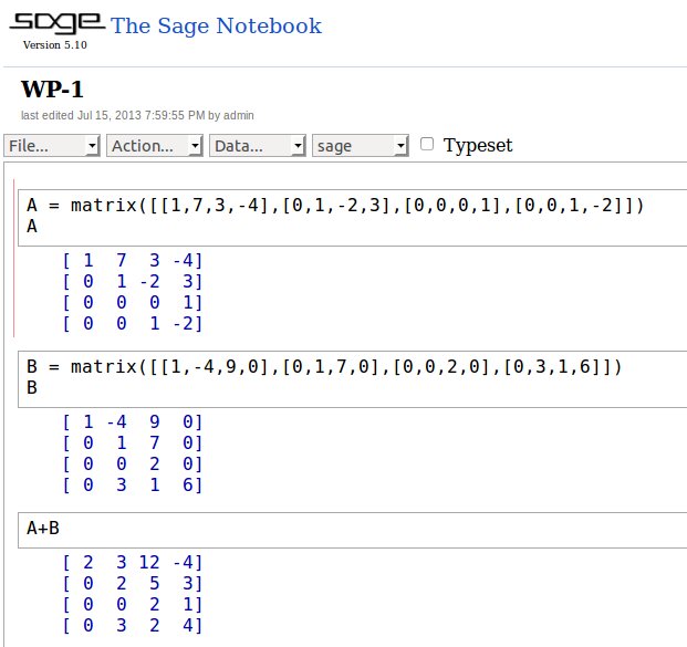
Here, you can see three cells of code along with output for each one. The first cell contains two commands, one to declare a matrix A, and another to show it:

\[A=\left[ \begin{array}{rrrr} 1 & 7 & 3 & -4\\0 & 1 & -2 & 3 \\0 & 0 & 0 & 1 \\ 0 & 0 & 1 & -2 \end{array} \right] \]

The second cell declares and prints matrix B:

\[B=\left[ \begin{array}{rrrr} 1 & -4 & 9 & 0\\0 & 1 & 7 & 0\\0 & 0 & 2 & 0\\0 & 3 & 1 & 6 \end{array} \right] \]

The third cell adds the two matrices together:

\[A+B=\left[ \begin{array}{rrrr} 1 & 7 & 3 & -4\\0 & 1 & -2 & 3 \\0 & 0 & 0 & 1 \\ 0 & 0 & 1 & -2 \end{array} \right]+\left[ \begin{array}{rrrr} 1 & -4 & 9 & 0\\0 & 1 & 7 & 0\\0 & 0 & 2 & 0\\0 & 3 & 1 & 6 \end{array} \right]=\left[ \begin{array}{rrrr} 2 & 3 & 12 & -4\\0 & 2 & 5 & 3\\0 & 0 & 2 & 1\\0 & 3 & 2 & 4 \end{array} \right]\]

Vector Addition

I really like Sage’s plotting capabilities. The following example declares two vectors, v1 and v2, and plots their sum, which is also a vector. v1 is blue, v2 is red, and the vector sum is purple:

SageNb4


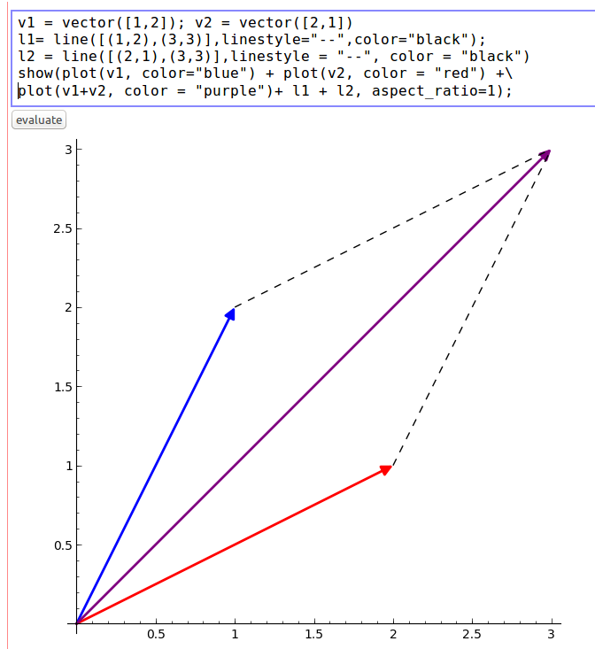
I added some dashed lines (which are declared as l1 and l2 in the cell) to complete the parallelogram in the plot. This shows that the sum of two vectors can be represented as the fourth vertex of the parallelogram where the other three vertices are its component vectors and the origin.

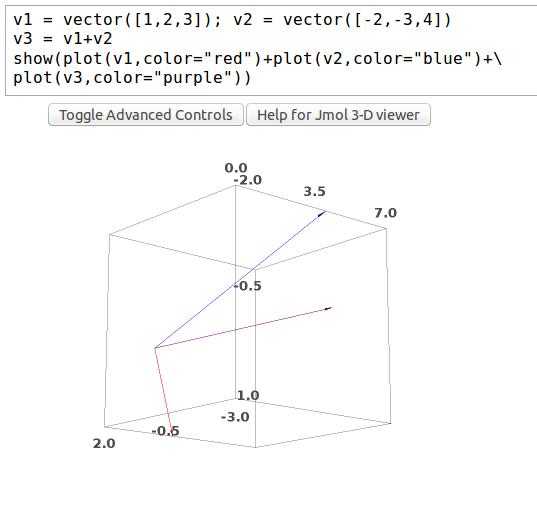
Sage also has 3D plotting capabilities. The following example shows the sum of two vectors in three-space along with its components:

SageNb5

Posted in: Logs, Mathematics / Tagged: david lay linear algebra, introduction to linear algebra, linear algebra, sagemath, serge lang, vector plot sage

No. 88: Communicating Mathematics via LaTeX

17 June, 2013 8:40 PM / Leave a Comment / Gene Dan

I started learning LaTeX a couple of years ago, but it wasn’t until last year when I started studying for actuarial exams 4/C and 3/MFE that I really started to become proficient at using it. If you are not familiar with what LaTeX is, it’s a markup language that lets you easily (although it takes some effort to learn) write mathematical formulas on a computer screen by using the keyboard. For example, \[ f(x) = \frac{1}{\sigma\sqrt{2\pi}}\mathrm{e}^{-\frac{(x-\mu)^2}{2\sigma^2}} !\], which is the code written in the WordPress editor, produces the formula for the Normal Distribution:

\[ f(x) = \frac{1}{\sigma\sqrt{2\pi}}\mathrm{e}^{-\frac{(x-\mu)^2}{2\sigma^2}} \]

You can try to write the above formula by using Microsoft Equation editor (like many of us did as highschoolers), but you’ll quickly realize that it takes an extremely long time, and you’ll be wishing that you had a faster, more efficient way of writing mathematical notation – this is where the usefulness of LaTeX becomes apparent.

I started using LaTeX while posting in the actuarial message boards, which are popular amongst candidates who are trying to study for exams. The bulletin board system has a LaTeX compiler installed, so you can easily consult other students from all across the world. For example, if I’m studying at 2:00 AM in the morning, I can post a question on the message board and there will most likely be someone who is awake at that time in Europe or China who would be willing to answer that question.

There are some more well-known message boards as well, such as StackOverflow and MathOverflow, where people (mostly from technical backgrounds) ask each other questions. Oftentimes they’ll use LaTeX to write technical notation – which greatly facilitates communication. I’ve found StackOverflow to be very helpful from time to time. On the other hand, I can’t even understand most of the questions being asked in MathOverflow, which is an online community of mathematicians asking each other research-level questions pertaining to mathematics. Fortunately, there’s another site under the StackExchange umbrella called Mathematics Stack Exachange, which caters to undergraduate and early graduate-level students, and is much more accessible. These websites are only 4 years old and have already made a huge impact on the way people collaborate on technical projects. I’m not sure if Don Knuth imagined this when he invented TeX way back in 1978, but if he did, he had tremendous foresight.

I’ll close by demonstrating a problem on matrices, which I started studying last week. I covered the basic row operations on matrices and today I just went over spanning and matrix equations in the Ax=b form. It’s been very interesting going back to material that I first learned 5 years ago – I have a different perspective now and it’s much like watching a movie – you always pick up something new the second time around.

Problem:

Solve the system of equations:

\[\begin{aligned} x_1 – 3x_3 &= 8 \\ 2x_1 + 2x_2 +9x_3 &= 7 \\ x_2 + 5x_3 &= -2 \end{aligned}\]

Solution:

We’ll start by writing the augmented matrix of this system of equations:

\[\left[ \begin{array}{rrrr} 1 & 0 & -3 & 8 \\ 2 & 2 & 9 & 7 \\ 0 & 1 & 5 & -2 \end{array} \right] \]

Replace row 2 with the sum of row 2 and negative 2 times row 1:

\[\left[ \begin{array}{rrrr} 1 & 0 & -3 & 8 \\ 0 & 2 & 15 & -9 \\ 0 & 1 & 5 & -2 \end{array} \right] \]

Interchange rows 2 and 3:

\[\left[ \begin{array}{rrrr} 1 & 0 & -3 & 8 \\ 0 & 1 & 5 & -2 \\ 0 & 2 & 15 & -9 \end{array} \right] \]

Replace row 3 with the sum of row 3 and negative 2 times row 2:

\[\left[ \begin{array}{rrrr} 1 & 0 & -3 & 8 \\ 0 & 1 & 5 & -2 \\ 0 & 0 & 5 & -5 \end{array} \right] \]

Scale row 3 by 1/5:

\[\left[\begin{array}{rrrr} 1 & 0 & -3 & 8 \\ 0 & 1 & 5 & -2 \\ 0 & 0 & 1 & -1 \end{array} \right] \]

Replace row 2 with the sum of row 2 and negative 5 times row 3:

\[\left[\begin{array}{rrrr} 1 & 0 & -3 & 8 \\ 0 & 1 & 0 & 3 \\ 0 & 0 & 1 & -1 \end{array} \right] \]

Replace row 1 with the sum of row 1 and three times row 3:

\[\left[\begin{array}{rrrr} 1 & 0 & 0 & 5 \\ 0 & 1 & 0 & 3 \\ 0 & 0 & 1 & -1 \end{array} \right] \]

This final matrix is equivalent to the following system of equations:

\[\begin{aligned} x_1 &= 5 \\ x_2 &= 3 \\ x_3 &= -1 \end{aligned} \]

Thus the solution set is \((5,3,-1)\)

The example above is how I would typically ask or answer a question posted on a bulletin board. Actually, giving out the entire solution (as above) is typically frowned upon and most people just give enough hints so that the person who asked the question can figure it out on their own. However, you can definitely see from the example that LaTeX allows you to cleanly print the matrices, which makes it much easier to understand. I remember back in high school when my friends and I would struggle trying to help each other out via AIM or some other chat client. I only wish I’d found out about LaTeX sooner.

Posted in: Logs, Mathematics / Tagged: LaTeX, mathoverflow, matrices, matrix, row operations, stackoverflow

No. 85: Things I’ve Been Doing Lately

10 June, 2013 9:40 PM / Leave a Comment / Gene Dan

I haven’t written in here for a long time, so I’d like to list what I’ve been doing these past few months to get the ball rolling:

Databases:

I took an interest in the study of databases late last year, and I’ve gotten a little further by studying the underlying concepts of database design and data modeling. I took the initiative to learn the subject after struggling with the technical aspects of my job. Last year, when I was first working with generalized linear models, I quickly found out that I couldn’t design the queries necessary to get the data I needed, and that I couldn’t communicate effectively with the IT personnel who were responsible for implementing my pricing models (in this case, implementation means to program the database systems that the business uses to store and capture information). Whenever I would ask them something, they would respond via their language of choice, T-SQL, which I had seen glimpses of during my internship days but couldn’t understand. At that time, I only had a vague notion of what a relational database was, and that it was somehow fundamentally different from an Excel spreadsheet, although I didn’t know why; if you ask me today I’d be able to tell you some of the fundamental differences – such as how a database has strictly defined fields and entity relationships, whereas Excel does not, etc. (well you could design an Excel spreadsheet to have those features, but it’s impractical).

This was perhaps the first time I thought to myself that maybe learning about databases would be important. I took a look at some books on SQL and another one that a co-worker checked out of the library, and determined that it would take me many months, if not a few years of investment to acquire proficiency in the subject. I encounter unfamiliar software and bits of code on a daily basis, so I often have to make the decision on whether or not I should spend a significant amount of time studying a software suite or language, or if I should just learn enough of it to complete my next assignment. For example, sometimes (about once every six months or so) I have to run some obsolete legacy software that I know will soon be replaced in the near future, so I’ll decide to learn just enough to get what I need. On the other hand, I see articles almost every single week pertaining to either SQL or relational databases on Hacker News, and several of my friends at coder meetup groups (which I’ll explain in the next section) use databases or write code pertaining to them, so I saw this as another sign that studying the subject would be worthwhile.

If you are not familiar at all with what I’m talking about, you may have seen stories in the news about cybercriminals (ranging from teenage misfits to professional cybersoldiers) infiltrating corporate and government databases, and you may have heard or seen the phrase “SQL Injection” thrown around in the technology section of newspapers. These concepts pertain to databases, which serve as centralized repositories for storing important information for businesses and governments. Prior to working in the corporate sector, news stories such as these were the only exposure I had to databases, and perhaps Americans who are working in non-technical jobs have a similar level of exposure, if any, at all. I think the media sensationalizes cybercrime because it deals with technology and concepts that the average citizen finds esoteric. I think perhaps stories like these, along with recent revelations during the past week should alert you to the importance of not only databases but also computer and technological literacy itself. I have some opinions on the matter but I believe that they are not yet mature enough for full disclosure now (maybe later), other than my belief that our nation is in a very precarious situation pertaining to civil liberties and privacy – and that our technological literacy is crucial to protecting ourselves from oppression. Perhaps this was the reason that influenced me to study databases seriously, or maybe it was really because I thought it would be important for work, I’m not so sure.

Anyway, I started getting some assignments at work done by first learning basic SELECT queries and joins, which allowed me to manipulate the data into the format I needed for my models. Lately, I’ve been looking in to theories on database design, which at least in my impression seems like some kind of applied set theory. I’ve also gotten involved in some open-source project dealing with databases, which I won’t reveal at this moment (maybe later). All I have to say is that I’m pretty excited to be working on something worthwhile.

Computer User Groups

I joined about 10 computer user groups on meetup.com. These user groups are weekly or monthly gatherings of people who want to talk about interests they have in common – such as music, sports, and various other hobbies. In my case, I’ve joined groups that discuss Python, Big Data, Perl, Linux, and Machine Learning that meet on a monthly basis. I’ve only been to the Python one so far, but I’m planning on going to a machine learning gathering in a few weeks. I’ve met some really cool people and learned a lot via these meetups.

Linear Algebra

I think a couple years ago I wrote about reviewing the mathematics that I learned in high school, and you may have noticed that on my “Readings” page, I’ve been stuck on my College Algebra book at 18.9% over the past 2 years. In that time I hadn’t stopped learning mathematics – I passed 3 actuarial exams in that time. However, now that I’m done with the preliminary exams I’m reluctant to go back to it, as when I was reviewing basic algebra, I was so bored going over things I had learned in the past and wasn’t patient enough to sit through it to make steady progress. Furthermore, I felt like I was spending so much time reviewing that I couldn’t devote enough effort to learning the new mathematics that I’m interested in. Therefore, I’ve decided to limit my “reviewing” to about 30 minutes a night, but make it mandatory. The rest of my time will be devoted to databases and linear algebra.

I took an intense course in Linear Algebra over a five-week span and did well, but due to the short time over which I learned the material (and the fact that it’s been 5 years since I took the course), I’ve forgotten most of it. However,  I’ve seen matrices appear more and more often in papers and in the work I’ve been doing (a computer uses matrix calculations to perform linear regression), so I decided to brush up on my linear algebra. This is technically a review, but since I spent a such a short time on the course the first time, I consider the material “new” enough to count as furthering my studies of mathematics. I also found the course very enjoyable, so I think this will give me a fresh perspective as I fill the gaps in my early education (after college algebra, I plan to review geometry, trig, and calculus) alongside the study of this subject.

Advances in computing power have only recently allowed us to realize the power of statistical matrix computations on large data sets. Matrices have been around for centuries, and Statistics has been around for centuries, but large organizations were not, at least until a few years ago, able to practically perform statistical calculations on data sets, nor did they have the technological capability to digitally store the data in their systems to make such calculations possible. Now that we can, a new field called data science is emerging, and it’ll play a crucial role in society in the near future (perhaps “data science” and “big data” are just buzzwords – it’s really just applied statistics).

I’d like to close with a simple demonstration on how a system of linear equations can be represented as a matrix:

\[ \begin{array}{rrrrrrr} x_1&-&2x_2&+&x_3&=&9 \\ &&2x_2&-&8x_3&=&8 \\ -4x_1&+&5x_2&+&9x_3&=&-9 \end{array}\]
can be represented as the augmented matrix:

\[ \left[\begin{array}{rrrr}1&-2&1&0\\ 0&2&-8&8 \\-4&5&9&-9\end{array}\right] \]

The properties of matrices allow us to sovlve systems of equations like these very efficiently. This particular example isn’t anything special, but I just wanted to show off the new LaTeX package I installed after switching to self-hosting. I think it’s much better than the default plugin used by wordpress.com – and I can even choose which one to use. This package is powered by MathJax which I think displays the formulas much more elegantly and cleanly than before. In addition, you can highlight each component of each formula, which is an improvement over what I had been using before. I’m satisfied with this plugin, although typing the above example was kind of a pain because the WordPress syntax for LaTeX expressions is a little different than what you would use for TeXLive. Actually, I think the terms in the equations above are too spaced out for my taste. I tried using the {align} environment but it came out weird, so I settled for the {array} environment. Maybe I’ll change it later.

I also have a new theme installed, which I like better than the temporary substitute I used last week. I think I’ll keep this one for now.

Posted in: Logs, Mathematics / Tagged: databases, python, relational databses, SQL

No. 83: Basic Simulation Using R

13 March, 2013 2:00 AM / Leave a Comment / Gene Dan

Today I’d like to demonstrate a few examples of simulation by using R’s built-in pseudorandom number generator. We’ll start by calling the function runif(n), which returns a vector of n draws from the uniform distribution on the interval [0,1]. To see what I mean, runif(50) will return 50 random numbers between 0 and 1 (inclusive):

[code language=”r” wraplines=”FALSE”]> runif(50)
[1] 0.79380213 0.02640186 0.48848994 0.50689348 0.27242565 0.37866590 0.50134423 0.04855088 0.35709235 0.06587394 0.04107046 0.52542577 0.31302174
[14] 0.65262709 0.60967237 0.45131387 0.55305078 0.83903314 0.72698109 0.06292518 0.47579002 0.15186000 0.71345801 0.71252703 0.22304757 0.20179550
[27] 0.57375115 0.06144426 0.87460214 0.87085905 0.52197596 0.79827053 0.35533929 0.23212775 0.30441290 0.29824819 0.59430450 0.92366848 0.63523013
[40] 0.59757710 0.67266388 0.06165364 0.12924342 0.10372910 0.49521401 0.31687057 0.08331765 0.51155404 0.35502189 0.65212223
[/code]

Interestingly, the numbers generated above aren’t actually random. R uses a process called pseudorandom number generation, which uses an algorithm to generate a long string of deterministic digits that appear to be random to most people, unless they have godlike powers of pattern recognition. The algorithm acts upon an initial value, called a seed, and for each seed the algorithm will return the same sequence of numbers. The term period refers to how long the sequence can go before it repeats itself. For example, Microsoft Excel’s PRNG (pseudorandom number generator) has a relatively short period, as (depending on the application) the sequence of numbers will repeat itself unless you frequently re-seed the algorithm. That is, if you generate a sequence 938745…, you’ll see 938745… again without too many draws.

The default PRNG used by R is called the Mersenne Twister, an algorithm developed in 1998 by Matsumoto and Nishimura. Other choices are available, such as Wichman-Hill, Marsaglia-Multicarry, Super-Duper, Knuth-TAOCP, and L’Ecuyer-CMRG. You can even supply your own PRNG, if you wish.

We can plot a histogram of a vector of generated numbers in order to observe the distribution of our sample. Below, you’ll see a 4-plot panel depicting samples from a uniform distribution on [0,1], with different draws per sample:

[code language=”r”]
#Uniform Sampling
par(mfrow=c(2,2))
for(i in 1:4){
x <- runif(10**i)
hist(x,prob=TRUE, col=”grey”,ylim=c(0,2),main = paste(10**i,” Draws”))
curve(dunif(x),add=TRUE,col=”red”,lwd=2)}
[/code]

unif

As you can see, the sample approaches the uniform distribution as the number of draws becomes larger.

Similarly, we can simulate observations from the normal distribution by calling the function rnorm(n,mean,sd), which returns a vector of n draws from the normal distribution with mean=mean and standard deviation = sd:

[code language=”r”]
#Normal Sampling
par(mfrow=c(2,2))
for(i in 1:4){
x <- rnorm(10**i)
hist(x,prob=TRUE,col=”grey”,ylim=c(0,.6),xlim=c(-4,4),main=paste(10**i,” Draws”))
curve(dnorm(x),add=TRUE,col=”red”,lwd=2)}
[/code]

norm4Likewise, as the number of draws gets bigger, the sample approaches the normal distribution.

We can use R to demonstrate the binomial approximation to the normal distribution. The binomial distribution with parameters n and p is approximately normal with mean np and variance np(1-p), with n large and p not too small. We’ll draw from the binomial distribution with n = 50 and p = .5, and then plot a normal curve with mean = 25 and variance = 12.5. Notice that as we increase the number of draws, the histrogram looks more and more like the normal distribution:

[code language=”r”]
#Binomial approximation to Normal
par(mfrow=c(2,2))
n <- 50
p <- .5
for(i in 1:4){
x <- rbinom(10**i,n,p)
hist(x,prob=TRUE,col=”grey”,ylim=c(0,.2),xlim=c(10,40),main=paste(10**i,” Draws”))
curve(dnorm(x,n*p,sqrt(n*p*(1-p))),add=TRUE,col=”red”,lwd=2)}
[/code]

binom_approx

For fun, I decided to see how many simulated values my computer could handle. I created a vector of 1 billion draws from the standard normal distribution:

[code language=”r”]
x<-rnorm(1000000000)
hist(x,prob=TRUE,col=”grey”,main=”1000000000 Draws”)
curve(dnorm(x),add=TRUE,col=”red”,lwd=2)
[/code]

norm5

Which took about 20 minutes to execute, using almost all of my computer’s memory (16 GB). This was unnecessary, as I could have reproduced the image above without as many draws. Nevertheless, I’m very impressed with R’s capabilities, as a similar script would have been impossible in Excel if I wanted to store the numbers in memory, or it would have taken much longer if I had even decided to clear the memory throughout the routine.

Posted in: Logs, Mathematics / Tagged: binomial approximation to normal, prng, pseudo random number generator, pseudorandom number generation, R, random number generator, simulation

No. 82: Plotting Normal Distributions with R

12 March, 2013 3:03 AM / 1 Comment / Gene Dan

Hey everyone,

I’ve got some good news  – I passed CA2 a few weeks ago and I’m glad I was able to knock out that requirement shortly after I passed CA1. The bad news is that I’ve only written three posts this year when I should have had ten, so I’ve got some catching up to do. Over the past couple of months, I’ve mostly been studying material related to the insurance industry, but I try to squeeze in some math or programming whenever I have time. Lately, I’ve been learning how to work with the SQL Server Management Studio interface to aggregate large datasets at work. For statistics, I’ve continued my studies with Verzani’s Using R for Introductory Statistics, which I started reading last year, but put off until this year due to exams. Today, I’d like to show you some of R’s plotting capabilities – we’ll start off with a plot of the standard normal distribution, and I’ll demonstrate how you can change the shape of the plotted distribution by adjusting its parameters.

If you’ve taken statistics, you’re most likely familiar with the normal distribution:

\[ f(x) = \frac{1}{\sigma\sqrt{2\pi}}\mathrm{e}^{-\frac{(x-\mu)^2}{2\sigma^2}} \]

One of the nice things about this distribution is that its two parameters are the mean and variance, which are common statistics used in everyday language. The mean is the average, a measure of central tendency that describes the center of the distribution, and the variance is a statistic that describes the spread of the distribution – how widely the data points deviate from the mean. The following code generates a plot of the density function of a standard normal random variable, and then adds two curves that depict the same distribution shifted to the left:

[code language=”r”]
#Standard normal, then shifted to the left
x <- seq(-6,6,length=500)
plot(x,dnorm(x,mean=0,sd=1),type = “l”,lty=1,lwd=3,col=”blue”,main=”Normal Distribution”,ylim=c(0,0.5),xlim=c(-6,6),ylab=”Density”)
curve(dnorm(x,-1,1),add=TRUE,lty=2,col=”blue”)
curve(dnorm(x,-2,1),add=TRUE,lty=3,col=”blue”)
legend(2,.5,legend=c(“N ~ (0, 1)”,”N ~ (-1, 1)”,”N ~ (-2, 1)”),lty=1:3,col=”blue”)
[/code]

norm1The code first generates a vector of length 500. This vector is then used as an argument to the dnorm() function, which returns the normal density of each element of the input vector. Notice that in line 2, dnorm(x,mean=0,sd=1) is a function with 3 arguments – the first specifies the input vector, the second specifies that the mean of the distribution equals 0, and the third argument specifies that the standard deviation of the distribution equals 1. The function returns a vector of densities which are in turn used as an input to the plot() function, which generates the solid blue line in the above figure. The next two lines of the script add the same distribution shifted 1 and 2 units to the left. You can see that in these two lines, the 2nd argument of the dnorm() function is -1 and -2, respectively – this means that I changed the mean of the distribution to -1 and -2, from 0, causing the leftward shift that you see above.

Similarly, I can shift the distribution to the right by increasing the mean:

[code language=”r”]
#Standard normal, then shifted to the right
x <- seq(-6,6,length=500)
plot(x,dnorm(x,mean=0,sd=1),type = “l”,lty=1,lwd=3,col=”purple”,main=”Normal Distribution”,ylim=c(0,0.5),xlim=c(-6,6),ylab=”Density”)
curve(dnorm(x,1,1),add=TRUE,lty=2,col=”purple”)
curve(dnorm(x,2,1),add=TRUE,lty=3,col=”purple”)
legend(-5.5,.5,legend=c(“N ~ (0, 1)”,”N ~ (1, 1)”,”N ~ (2, 1)”),lty=1:3,col=”purple”)
[/code]

norm2

Notice that I can change the position of the legend by specifying the x and y coordinates in the first two arguments of the legend() function.

The next script keeps the mean at 0, but adds two curves with the standard deviation increased to 1 and 2:

[code language=”r”]
#Standard normal, then increased variance
x <- seq(-6,6,length=500)
plot(x,dnorm(x,mean=0,sd=1),type = “l”,lty=1,lwd=3,col=”black”,main=”Normal Distribution”,ylim=c(0,0.5),xlim=c(-6,6),ylab=”Density”)
curve(dnorm(x,0,1.5),add=TRUE,lty=2,col=”red”)
curve(dnorm(x,0,2),add=TRUE,lty=3,col=”black”)
legend(-5.5,.5,legend=c(“N ~ (0, 1)”,”N ~ (0, 2.25)”,”N ~ (0, 4)”),lty=1:3,col=c(“black”,”red”,”black”))
[/code]

norm3

Here, I made the middle curve red by using the “col” argument in the plot() function. Personally, plotting is one of my favorite things to do with R. I feel that visualizing data helps you gain an intuitive grasp on the subject, and reveals patterns that you might not otherwise see with aggregated tables or simple summary statistics. Later on this week (hopefully tomorrow), I’ll demonstrate some simple simulations with the normal distribution.

Posted in: Logs, Mathematics / Tagged: cran, normal plot r, R

Post Navigation

« Previous 1 … 5 6 7 8 9 10 Next »

Archives

  • September 2023
  • February 2023
  • January 2023
  • October 2022
  • March 2022
  • February 2022
  • December 2021
  • July 2020
  • June 2020
  • May 2020
  • May 2019
  • April 2019
  • November 2018
  • September 2018
  • August 2018
  • December 2017
  • July 2017
  • March 2017
  • November 2016
  • December 2014
  • November 2014
  • October 2014
  • August 2014
  • July 2014
  • June 2014
  • February 2014
  • December 2013
  • October 2013
  • August 2013
  • July 2013
  • June 2013
  • March 2013
  • January 2013
  • November 2012
  • October 2012
  • September 2012
  • August 2012
  • July 2012
  • June 2012
  • May 2012
  • April 2012
  • March 2012
  • February 2012
  • January 2012
  • December 2011
  • September 2011
  • August 2011
  • July 2011
  • June 2011
  • January 2011
  • December 2010
  • October 2010
  • September 2010
  • August 2010
  • June 2010
  • May 2010
  • April 2010
  • March 2010
  • September 2009
  • August 2009
  • May 2009
  • December 2008

Categories

  • Actuarial
  • Cycling
  • Logs
  • Mathematics
  • MIES
  • Music
  • Uncategorized

Links

Cyclingnews
Jason Lee
Knitted Together
Megan Turley
Shama Cycles
Shama Cycles Blog
South Central Collegiate Cycling Conference
Texas Bicycle Racing Association
Texbiker.net
Tiffany Chan
USA Cycling
VeloNews

Texas Cycling

Cameron Lindsay
Jacob Dodson
Ken Day
Texas Cycling
Texas Cycling Blog
Whitney Schultz
© Copyright 2025 - Gene Dan's Blog
Infinity Theme by DesignCoral / WordPress