• Home
  • Readings
  • Github
  • MIES
  • TmVal
  • About
Gene Dan's Blog

Category Archives: Mies

No. 138: MIES – Offer, Engel, and Personal Demand Curves

14 June, 2020 10:11 PM / Leave a Comment / Gene Dan


This entry is part of a series dedicated to MIES – a miniature insurance economic simulator. The source code for the project is available on GitHub.

Current Status

Last week, I specified a Cobb Douglas utility curve for each person in MIES. I also demonstrated a situation in which a person might choose to not fully insure. However, I’ve gone a few chapters ahead in my readings and found out that under certain assumptions, a risk-averse person who is offered a fair premium will choose to fully insure. In MIES, since each company charges the pure premium without loading for profit or expenses, each person is getting a fair premium – so there’s something missing from my current model that makes it inconsistent with economic theory.

Risk aversion is not yet implemented in MIES, and will have to wait a few weeks before I get to it, since there’s quite a bit of work to do. But I’m mentioning the issue here, just in case someone reading this knows more about the subject than I do.

This week, I’m going to demonstrate a set of tools to examine consumer choice – the offer, Engel, and personal demand curves. I don’t recall using the first two curves very much in my economics courses, but the latter will be very important and will serve as a bridge between personal demand and market demand. Surprisingly, these curves were very quick to implement, since they all rely on the same method I wrote last week for the Cobb Douglas class.

The topic of this post roughly corresponds to chapter 6 of Varian.

Offer Curve

The offer curve for a consumer depicts their optimal consumption bundle at each level of income. Since the offer curve is unique to a particular consumer, I decided to define the methods that generate and plot the offer curve within the Person class. Luckily, the CobbDouglas class that I defined last week has a method called optimal_bundle, which returns the optimal consumption bundle given a set of prices and income. Since this is exactly what we need given the definition of the offer curve, we can simply use this method to generate each person’s offer curve:

Python
1
2
3
4
5
6
7
8
9
10
    def get_offer(self):
        # only works for Cobb Douglas right now
        def o(m):
            return self.utility.optimal_bundle(
                p1=self.premium,
                p2=1,
                m=m
            )
 
        self.offer = o

Note that while I only have one utility curve defined in MIES at the moment (Cobb Douglas), the definition of the offer curve doesn’t need to have anything specific to the Cobb Douglas utility function. This means in the future, I should be able to abstract this method to accept other utility functions without too much modification.

I’ve also added a method to plot a person’s offer curve:

Python
1
2
3
4
5
6
7
8
9
10
11
12
13
14
15
    def show_offer(self):
        offer_frame = pd.DataFrame(columns=['income'])
        offer_frame['income'] = np.arange(0, self.income * 2, 1000)
        offer_frame['x1'], offer_frame['x2'] = self.offer(offer_frame['income'])[:2]
 
        offer_trace = {
            'x': offer_frame['x1'],
            'y': offer_frame['x2'],
            'mode': 'lines',
            'name': 'Offer Curve'
        }
 
        fig = self.consumption_figure
        fig.add_trace(offer_trace)
        plot(fig)

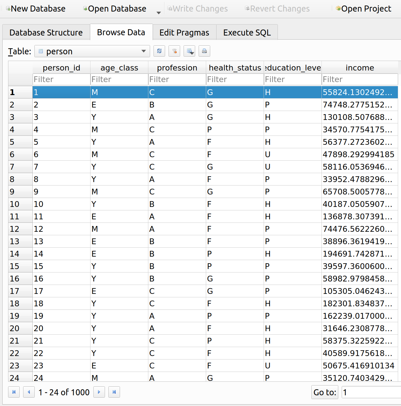
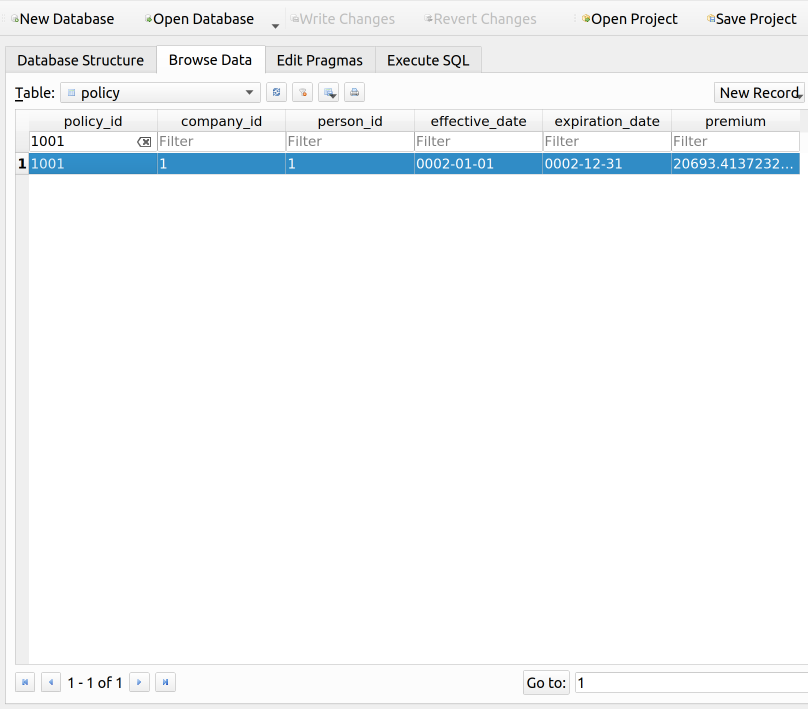
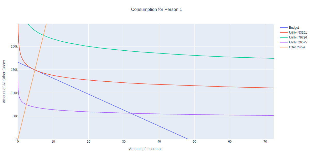
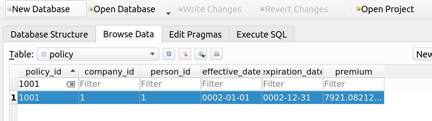
This method takes a preset range of income values, and uses the get_offer method to plot the optimal consumption bundle for each income value in the range. For example if we’ve already run a few iterations of a market simulation, we can examine what combinations of insurance and non-insurance a person can afford at different income levels. Let’s do this for the person with id=1:

1
2
3
4
5
6
7
8
my_person = Person(session=gsession, engine=engine, person=PersonTable, person_id=1)
my_person.get_policy(Policy, 1001)
 
my_person.get_budget()
my_person.get_consumption()
my_person.get_consumption_figure()
my_person.get_offer()
my_person.show_offer()

Imagine what would happen if you were to shift the blue budget line inward and outward. The optimal consumption bundle would the the point of tangency with the corresponding utility function. We can see that the orange offer curve is the set of all these points.

Engel Curve

The Engel curve is similar to the offer curve, but plots the optimal choice of a good at various levels of income. Its definition within the Person class is also similar, except we only need to return the first good of the optimal bundle:

Python
1
2
3
4
5
6
7
8
9
10
11
    def get_engel(self):
        # only works for Cobb Douglas right now
 
        def e(m):
            return self.utility.optimal_bundle(
                p1=self.premium,
                p2=1,
                m=m
            )[0]
 
        self.engel = e

1
2
3
4
5
6
7
8
9
10
11
12
13
14
15
16
17
18
19
20
21
22
23
24
25
26
27
    def show_engel(self):
        engel_frame = pd.DataFrame(columns=['income'])
        engel_frame['income'] = np.arange(0, self.income * 2, 1000)
        engel_frame['x1'] = engel_frame['income'].apply(self.engel)
 
        engel_trace = {
            'x': engel_frame['x1'],
            'y': engel_frame['income'],
            'mode': 'lines',
            'name': 'Engel Curve'
        }
 
        fig = go.Figure()
        fig.add_trace(engel_trace)
 
        fig['layout'].update({
            'title': 'Engel Curve for Person ' + str(self.id),
            'title_x': 0.5,
            'xaxis': {
                'title': 'Amount of Insurance'
            },
            'yaxis': {
                'title': 'Income'
            }
        })
 
        plot(fig)

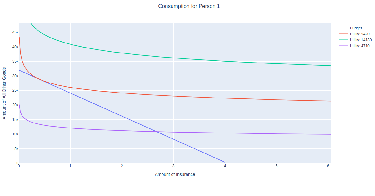
Let’s see what the Engel curve looks like for person 1:

1
2
3
4
5
6
7
8
9
my_person = Person(session=gsession, engine=engine, person=PersonTable, person_id=1)
my_person.get_policy(Policy, 1001)
my_person.premium
my_person.get_budget()
my_person.get_consumption()
my_person.get_consumption_figure()
 
my_person.get_engel()
my_person.show_engel()

Demand Curve

The demand function depicts how much of a good a person would buy if it were at a certain price. This one’s important since we’ll need it to derive industry demand, which will then be used to answer many fundamental questions about the insurance market. Like the other curves, defining this one was simple, we just get the optimal bundle at each price and return the quantity demanded of the first good:

Python
1
2
3
4
5
6
7
8
9
10
11
    def get_demand(self):
        # only works for Cobb Douglas right now
 
        def d(p):
            return self.utility.optimal_bundle(
                p1=p,
                p2=1,
                m=self.income
            )[0]
 
        self.demand = d

Python
1
2
3
4
5
6
7
8
9
10
11
12
13
14
15
16
17
18
19
20
21
22
23
24
25
26
27
28
    def show_demand(self):
        demand_frame = pd.DataFrame(columns=['price'])
        demand_frame['price'] = np.arange(self.premium/100, self.premium * 2, self.premium/100)
        demand_frame['x1'] = demand_frame['price'].apply(self.demand)
 
        demand_trace = {
            'x': demand_frame['x1'],
            'y': demand_frame['price'],
            'mode': 'lines',
            'name': 'Demand Curve'
        }
 
        fig = go.Figure()
        fig.add_trace(demand_trace)
 
        fig['layout'].update({
            'title': 'Demand Curve for Person ' + str(self.id),
            'title_x': 0.5,
            'xaxis': {
                'range': [0, self.income / self.premium * 2],
                'title': 'Amount of Insurance'
            },
            'yaxis': {
                'title': 'Premium'
            }
        })
 
        plot(fig)

Let’s see what the demand curve looks like for person 1:

1
2
3
4
5
6
7
8
9
10
my_person = Person(session=gsession, engine=engine, person=PersonTable, person_id=1)
my_person.get_policy(Policy, 1001)
my_person.premium
my_person.get_budget()
my_person.get_consumption()
my_person.get_consumption_figure()
my_person.get_offer()
 
my_person.get_demand()
my_person.show_demand()

Note that the demand curve slopes downward as it should, since we’d expect a person to buy more insurance the cheaper it is. However, note that there is no price such that the demand equals zero. The demand curve asymptotically approaches zero as the premium increases, but this particular person will never go uninsured. This is due the property of the Cobb Douglas utility function that the exponent of the good equals the percent of income spent on that good, which is hard coded as 10% at the moment. However, in the real world people do go uninsured, and this is a subject of great interest to me, so we’ll need to revisit this later.

Further Improvements

I’ve added quite a few features to the person class, but I haven’t integrated them to the point where I can perform more than two market simulations. I’m also several chapters ahead in my readings than what I’ve posted about, and I’ve encountered an interesting demonstration on risk aversion and intertemporal choice concerning assets, which will take quite an effort to both implement and reconcile with what I’ve written so far.

Posted in: Actuarial, Mathematics, MIES

No. 137: MIES – Cobb-Douglas Utility

7 June, 2020 3:30 PM / Leave a Comment / Gene Dan


This entry is part of a series dedicated to MIES – a miniature insurance economic simulator. The source code for the project is available on GitHub.

Current Status

Last week, I demonstrated how MIES can be used to calculate the budget constraint for each insured in the marketplace. This answered the question – how much insurance can each person afford during each underwriting period?

Although we now have the set of all possible consumption bundles that each person can afford, we still have no method for determining what bundle they will ultimately select – that is, how much insurance will each person actually buy? To answer this question, we turn to the concept of utility. Utility is a measurement of the satisfaction a person receives from a course of action, and we will assume that rational people seek to maximize their utility under scarcity. In this case, the course of action is purchasing insurance, and people seek to maximize their utility subject to the constraint of what they can afford.

Thus, for today’s post I will demonstrate how MIES can assign a utility function to each person in the market and determine each how much insurance each person will purchase.

By introducing utility, I would eventually like to answer certain questions I had about the insurance industry when I thought about building MIES. None of these will be answered today, but this should take us one step closer:

  1. How much insurance will be purchased in total at market equilibrium?
  2. Who will go uninsured?
  3. Should there be a mandatory minimum amount of insurance required by law? If so, should there be a state-run high-risk pool? And if so, how should it be funded?

More detailed treatment of utility can be found in chapters 4 and 5 of Varian.

Utility

To model each person’s preferences for insurance consumption, I’ve decided to use the Cobb-Douglas utility function:

    \[u(x_1, x_2) = x_1^c x_2^d\]

Where c and d represent the percentage of income spent on goods x_1 and x_2 when c + d = 1, and each x represents the quantity of each good. While other utility functions may eventually prove to be more realistic for our simulation, Cobb-Douglas utility functions are a good candidate to start with since they have many convenient features. For example, in order to find the optimal consumption bundle for a person, we need to find the bundle of goods such that the marginal rate of substitution (MRS) equals the slope of the budget constraint, while satisfying the budget constraint itself. For the Cobb-Douglas utility function, Varian provides a derivation for the MRS:

    \[\text{MRS} = -\frac{\partial u(x_1, x_2) / \partial x_1}{\partial u(x_1, x_2) / \partial x_2} \]

This can then be used with the budget constraint, p_1 x_1 + p_2 x_2 = m, to solve for the quantities of x_1 and x_2 given the income and price of each good:

    \[x_1 = \frac{c}{c + d}\frac{m}{p_1}\]

    \[x_2 = \frac{d}{c + d} \frac{m}{p_2}\]

and, when c + d = 1, x_1 = cm / p_1 and x_2 = dm/p_2. This means that using this result, we can find the optimal consumption bundle algebraically. This is very useful since 1) I have simply forgotten a lot of calculus since leaving school and 2) I won’t have to program calculus into MIES for the time being.

The convexity of the Cobb-Douglas utility function also satisfies certain assumptions underlying consumer behavior. Chapter 3 of Varian provides an in-depth explanation of these assumptions.

Utility Module

I hinted last week that I thought it might be a good idea to break up the econtools.py module into more specific modules. I’ve decided to do this to improve readability and to keep things organized. I’ve created a new folder called econtools to house these modules. The Budget class is now in the budget.py module and the utility function classes are now in a file called utility.py.

The utility.py module contains a single class, called CobbDouglas:

Python
1
2
3
4
5
6
7
8
9
10
11
12
13
14
15
16
17
18
19
20
21
22
23
24
25
26
27
28
29
30
31
32
33
34
35
36
37
38
39
40
41
42
43
44
45
46
47
import plotly.graph_objects as go
import numpy as np
 
from plotly.offline import plot
 
 
class CobbDouglas:
 
    def __init__(self, c, d):
        self.c = c
        self.d = d
 
    def optimal_bundle(self, p1, p2, m):
        x1_quantity = (self.c / (self.c + self.d)) * (m / p1)
        x2_quantity = (self.d / (self.c + self.d)) * (m / p2)
 
        optimal_utility = (x1_quantity ** self.c) * (x2_quantity ** self.d)
 
        return x1_quantity, x2_quantity, optimal_utility
 
    def trace(self, k, m):
        x_values = np.arange(.01, m * 1.5,.01)
        y_values = (k/(x_values ** self.c)) ** (1/self.d)
 
        return {'x': x_values,
                'y': y_values,
                'mode': 'lines',
                'name': 'Utility: ' + str(int(round(k)))}
 
    def show_plot(self, k=5, m=10):
        fig = go.Figure(data=self.trace(k, m))
        fig.add_trace(self.trace(k * 1.5, m))
        fig.add_trace(self.trace(k * .5, m))
        fig['layout'].update({
            'title': 'Cobb Douglas Utility',
            'title_x': 0.5,
            'xaxis': {
                'range': [0, m * 1.5],
                'title': 'Amount of Good X'
            },
            'yaxis': {
                'range': [0, m * 1.5],
                'title': 'Amount of Good Y'
            },
            'showlegend': True
        })
        plot(fig)

The CobbDouglas class takes two arguments, c and d, which correspond to the c and d parameters in the function definition. The class provides three methods: optimal_bundle() calculates the optimal consumption bundle using the results derived by Varian, trace() defines the curve as it will appear when plotted, and show_plot() plots the utility function.

Here’s an example on how to use the class to plot the function:

Python
1
2
3
4
from econtools import CobbDouglas
 
corn_on_the_cobb = CobbDouglas(.5, .5)
corn_on_the_cobb.show_plot()

Here, we’ve provided a simple example where c = d = .5, which means that the consumer will allocate 50% of their income to each good. If the price of each good is the same, the line connecting all optimal consumption bundles will go through the origin (more on that for a later post).

MIES Integration

The Person Class

Now that we’ve got a class defined for our Cobb Douglas function, we now need to find a way to get it working with MIES. I’d like to be able to access the utility function for each consumer in the simulation. Since I’ve started to examine more person-specific characteristics, I’ve created a new class in the entities.py module, Person:

Python
1
2
3
4
5
6
7
8
9
10
11
12
13
14
15
16
17
18
19
20
21
22
23
24
25
26
27
28
29
30
31
32
33
34
35
36
37
38
39
40
41
42
43
44
45
46
47
48
49
50
51
52
53
54
55
56
57
58
59
60
61
62
63
64
65
66
67
68
69
70
71
72
73
74
75
76
77
78
79
80
81
82
83
84
85
86
87
88
class Person:
    def __init__(
        self,
        session,
        engine,
        person,
        person_id
    ):
        self.session = session
        self.connection = engine.connect()
        self.engine = engine
        self.id = person_id
 
        query = self.session.query(person).filter(
                person.person_id == int(self.id)
            ).statement
 
        self.data = pd.read_sql(
            query,
            self.connection
        )
        self.income = self.data['income'].loc[0]
 
        self.utility = CobbDouglas(
            c=self.data['cobb_c'].loc[0],
            d=self.data['cobb_d'].loc[0]
        )
 
        self.policy = None
        self.budget = None
        self.premium = None
        self.optimal_bundle = None
        self.consumption_figure = None
 
    def get_policy(
        self,
        policy,
        policy_id
    ):
        query = self.session.query(policy).filter(
            policy.policy_id == int(policy_id)
        ).statement
 
        self.policy = pd.read_sql(
            query,
            self.connection
        )
        self.premium = self.policy['premium'].loc[0]
 
    def get_budget(self):
        all_other = Good(1, name='All Other Goods')
        if self.policy is None:
            insurance = Good(4000, name='Insurance')
        else:
            insurance = Good(self.premium, name='Insurance')
        self.budget = Budget(insurance, all_other, income=self.income, name='Budget')
 
    def get_consumption(self):
        self.optimal_bundle = self.utility.optimal_bundle(
            p1=self.premium,
            p2=1,
            m=self.income
        )
 
    def get_consumption_figure(self):
        fig = go.Figure()
        fig.add_trace(self.budget.get_line())
        fig.add_trace(self.utility.trace(k=self.optimal_bundle[2], m=self.income / self.premium * 1.5))
        fig.add_trace(self.utility.trace(k=self.optimal_bundle[2] * 1.5, m=self.income / self.premium * 1.5))
        fig.add_trace(self.utility.trace(k=self.optimal_bundle[2] * .5, m=self.income / self.premium * 1.5))
 
        fig['layout'].update({
            'title': 'Consumption for Person ' + str(self.id),
            'title_x': 0.5,
            'xaxis': {
                'title': 'Amount of Insurance',
                'range': [0, self.income / self.premium * 1.5]
            },
            'yaxis': {
                'title': 'Amount of All Other Goods',
                'range': [0, self.income * 1.5]
            }
        })
        self.consumption_figure = fig
        return fig
 
    def show_consumption(self):
        plot(self.consumption_figure)

Since there is already a Person class in the schema.py module referencing a SQLite table, I’ve renamed that class to PersonTable. The Person class takes a database connection, along with the person table in the database, queries the details of a person, and generates a utility function for that person. The Person class provides additional methods for attaching policy information, calculating that person’s budget, and determining how much insurance they will buy.

To keep things simple, I’ve assumed that each person’s c parameter equals, .1, which means that the population has homogeneous preferences for insurance, and will spend 10% of their income on it. The parameters.py module and environment class have been updated accordingly to reflect this. We can loosen these assumptions later on.

Optimal Consumption

Let’s find one person’s optimal bundle for purchasing insurance. To do this, we run two iterations of the simulation and examine the results for person_id = 1, like we did last week:

Python
1
2
3
4
5
6
7
8
9
10
11
12
13
14
15
16
17
18
19
20
21
22
23
24
25
26
27
28
29
30
31
32
33
34
35
36
37
38
39
40
41
import pandas as pd
import datetime as dt
import sqlalchemy as sa
import econtools as ec
from SQLite.schema import PersonTable, Policy, Base, Company, Event
from sqlalchemy.orm import sessionmaker
from entities import God, Broker, Insurer, Person
import numpy as np
import plotly.graph_objects as go
from plotly.offline import plot
 
 
pd.set_option('display.max_columns', None)
 
 
engine = sa.create_engine('sqlite:///MIES_Lite.db', echo=True)
Session = sessionmaker(bind=engine)
Base.metadata.create_all(engine)
 
gsession = Session()
 
 
ahura = God(gsession, engine)
ahura.make_population(1000)
 
pricing_date = dt.date(1, 12, 31)
 
 
rayon = Broker(gsession, engine)
company_1 = Insurer(gsession, engine, 4000000, Company, 'company_1')
company_1_formula = 'severity ~ age_class + profession + health_status + education_level'
pricing_status = 'initial_pricing'
free_business = rayon.identify_free_business(PersonTable, Policy, pricing_date)
 
companies = pd.read_sql(gsession.query(Company).statement, engine.connect())
 
rayon.place_business(free_business, companies, pricing_status, pricing_date, company_1)
ahura.smite(PersonTable, Policy, pricing_date + dt.timedelta(days=1))
company_1.price_book(PersonTable, Policy, Event, company_1_formula)
pricing_status = 'renewal_pricing'
rayon.place_business(free_business, companies, pricing_status, pricing_date, company_1)

This person has an income of about 32k. You can also see additional columns for their Cobb Douglas parameters. If all goes well, we would expect them to want to spend about 3200 on insurance. Let’s query their renewal quote to see how much premium they need to pay:

Python
1
2
my_person = Person(session=gsession, engine=engine, person=PersonTable, person_id=1)
my_person.get_policy(Policy, 1001)

Since their premium is about 8k, we’d expect them to consume roughly 3.2/8 = .4 units of insurance upon renewal. Let’s solve for their optimal bundle to confirm:

Python
1
2
3
my_person.get_budget()
my_person.get_consumption()
my_person.get_consumption_figure()

Indeed, the point of tangency between the budget constraint and red utility curve is around .4 (ish) units of insurance. Interestingly, since the insured will only purchase .4 units of insurance upon renewal, they are no longer fully insured. From an actuarial standpoint, it is desirable for customers to fully insure things like homes, and a penalty is typically built into the premium if a customer decides not to do so. More on that topic (much) later.

Further Improvements

I’ve introduced quite a few concepts into the consumption aspect of MIES, and have yet to rerun the simulation for more than two iterations. Before I can do this, I’ll need to revise certain aspects of the insureds, such as personal wealth, and partial insurance. I have not even incorporated wealth for each person, so the idea of having only part of it covered under the case of partial insurance currently has no meaning.

Appendix: SymPy

Since the optimization problem discussed here involves calculus, I thought maybe I should eventually have some calculus programmed in MIES. There’s a library called SymPy that facilitates symbolic computation in Python. Let’s try it out by computing the partial derivatives of the Cobb-Douglas utility function, required to solve for the MRS:

Python
1
2
3
4
5
6
7
from sympy import symbols, diff
 
c, d, x1, x2 = symbols('c d x1 x2')
u = (x1 ** c) * (x2 ** d)
 
mrs = -diff(u, x1) / diff(u, x2)
print(mrs)

The console prints -c*x2/(d*x1), which is MRS = -\frac{c x_2}{d x_1}, the same as that derived in Varian. That looks pretty useful. However, Sympy’s documentation is massive, at over 2000 pages. It might take some time to learn it, even if it just involves me grabbing what I need. Since I can make do without calculus for the time being, I’ll save this for another day.

Posted in: Actuarial, Mathematics, MIES

No: 136: MIES – Personal Budget Constraints, Taxes, and Subsidies

2 June, 2020 9:08 PM / 1 Comment / Gene Dan

This entry is part of a series dedicated to MIES – a miniature insurance economic simulator. The source code for the project is available on GitHub.

Current Status

Last week, I demonstrated the first simulation of MIES. Although it can run indefinitely without intervention on my part, I’ve made a lot of assumptions that aren’t particularly realistic – such as the ability of insureds to buy as much insurance as they wanted without any kind of constraint on affordability. I’ll address this today by implementing a budget constraint, a concept typically introduced during the first week of a second year economics course.

Most of the economic theory that I’ll be introducing to MIES for the time being comes from two books: Hal Varian’s Intermediate Microeconomics, a favorite of mine from school, and Zweifel and Eisen’s Insurance Economics, which at least according to the table of contents and what little I’ve read so far, seems to have much of the information I’d want to learn about for MIES.

I’m going to avoid repeating much of what can already be read in these books, so just an fyi, these are the sources I’m drawing from. My goals are to refresh my knowledge of economics as I read and then implement what I see in Python to add features to MIES.

The Economics Module

I’ve added a new module to the project, econtools.py. For now, this will contain the classes for exploring economics concepts with MIES, but seeing how much it has grown in just one week, it’s likely I’ll break it up in the near future. I’ll go over the first classes I’ve written for the module, those written for the budget constraint: Budget, Good, Tax, and Subsidy.

Budget Constraint

Those of you who have taken an economics course ought to find the following graph, a budget constraint, familiar:

As in the real world, there are only two goods that a person can possibly buy:

  1. Insurance
  2. Non-insurance

The budget constraint represents the set of possible allocations between insurance and non-insurance, aka all other goods. This can be represented by an equation as well:

    \[p_1 x_1 + p_2 x_2 = m\]

Where each x represents the quantity of each good and each p represents the prices per unit for each good, and m represents income. People can only buy as much insurance as their incomes can support, hence the need for introducing this constraint into MIES for each person. The budget constraint simply shows that in order to buy one dollar more of insurance, you have to spend one dollar less on anything else that you were going to buy with your income.

The price of insurance is often thought of as a rate per unit of exposure, exposure being some kind of denominator to measure risk, such as miles driven, house-years, actuarial exams taken, or really anything you can think of that correlates with a risk that you’d like to charge money for.

Interestingly, there is nothing in the budget constraint as shown above that would prevent someone from insuring something twice or purchasing some odd products like a ‘lose-1-dollar-get-5-dollars back’ multiplier scheme. I’m not sure if these are legal or simply just discouraged by insurers as I’ve never tried to buy such a product myself or seen it advertised. I could imagine why insurers would not to sell these things – maybe due to the potential for fraud or the fact that an insured thing is 100% correlated with itself. On the other hand, a company might be able to compensate for these risks by simply charging more money to accept them. Regardless, if these products are really undesirable, I’d rather let the simulations demonstrate the impact of unrestricted product design than to have it constrained from the start. I’ll save that for another day.

The budget constraint is modeled with the Budget class in econtools.py. It accepts the goods to be allocated along with other relevant information, such as their prices and the income of the person for whom we are modeling the budget. You’ll see that the class contains references to the other component classes (Good, Tax, Subsidy) which are explained later:

Python
1
2
3
4
5
6
7
8
9
10
11
12
13
14
15
16
17
18
19
20
21
22
23
24
25
26
27
28
29
30
31
32
33
34
35
36
37
38
39
40
41
42
43
44
45
46
47
48
49
50
51
52
53
54
55
56
57
58
59
60
61
62
63
64
65
66
67
68
69
70
71
72
73
74
75
76
77
78
79
80
81
82
83
84
85
86
87
88
89
90
91
92
93
94
95
96
97
98
99
100
101
102
103
104
105
106
107
108
109
110
111
112
113
114
115
116
117
118
119
120
121
122
123
124
125
126
127
128
129
130
131
132
133
134
135
136
137
138
class Budget:
    def __init__(self, good_x, good_y, income, name):
        self.good_x = good_x
        self.good_y = good_y
        self.income = income
        self.x_lim = self.income / (min(self.good_x.adjusted_price, self.good_x.price)) * 1.2
        self.y_lim = self.income / (min(self.good_y.adjusted_price, self.good_y.price)) * 1.2
        self.name = name
 
    def get_line(self):
        data = pd.DataFrame(columns=['x_values', 'y_values'])
        data['x_values'] = np.arange(int(min(self.x_lim, self.good_x.ration)) + 1)
 
        if self.good_x.tax:
            data['y_values'] = self.calculate_budget(
                good_x_price=self.good_x.price,
                good_y_price=self.good_y.price,
                good_x_adj_price=self.good_x.adjusted_price,
                good_y_adj_price=self.good_y.adjusted_price,
                m=self.income,
                modifier=self.good_x.tax,
                x_values=data['x_values']
            )
        elif self.good_x.subsidy:
            data['y_values'] = self.calculate_budget(
                good_x_price=self.good_x.price,
                good_y_price=self.good_y.price,
                good_x_adj_price=self.good_x.adjusted_price,
                good_y_adj_price=self.good_y.adjusted_price,
                m=self.income,
                modifier=self.good_x.subsidy,
                x_values=data['x_values']
            )
        else:
            data['y_values'] = (self.income / self.good_y.adjusted_price) - \
                       (self.good_x.adjusted_price / self.good_y.adjusted_price) * data['x_values']
 
        return {'x': data['x_values'],
                'y': data['y_values'],
                'mode': 'lines',
                'name': self.name}
 
    def calculate_budget(
            self,
            good_x_price,
            good_y_price,
            good_x_adj_price,
            good_y_adj_price,
            m,
            modifier,
            x_values
    ):
        y_int = m / good_y_price
        slope = -good_x_price / good_y_price
        adj_slope = -good_x_adj_price / good_y_adj_price
        base_lower = int(modifier.base[0])
        base_upper = int(min(modifier.base[1], max(m / good_x_price, m / good_x_adj_price)))
        modifier_type = modifier.style
 
        def lump_sum(x):
            if x in range(modifier.amount + 1):
                x2 = y_int
                return x2
            else:
                x2 = y_int + adj_slope * (x - modifier.amount)
                return x2
 
        def no_or_all_adj(x):
            x2 = y_int + adj_slope * x
            return x2
 
        def beg_adj(x):
            if x in range(base_lower, base_upper + 1):
                x2 = y_int + adj_slope * x
                return x2
            else:
                x2 = y_int + slope * (x + (adj_slope/slope - 1) * base_upper)
                return x2
 
        def mid_adj(x):
            if x in range(base_lower):
                x2 = y_int + slope * x
                return x2
            elif x in range(base_lower, base_upper + 1):
                x2 = y_int + adj_slope * (x + (slope/adj_slope - 1) * (base_lower - 1))
                return x2
            else:
                x2 = y_int + slope * (x + (adj_slope/slope - 1) * (base_upper - base_lower + 1))
                return x2
 
        def end_adj(x):
            if x in range(base_lower):
                x2 = y_int + slope * x
                return x2
            else:
                x2 = y_int + adj_slope * (x + (slope/adj_slope - 1) * (base_lower - 1))
                print(x, x2)
                return x2
 
        cases = {
            'lump_sum': lump_sum,
            'no_or_all': no_or_all_adj,
            'beg_adj': beg_adj,
            'mid_adj': mid_adj,
            'end_adj': end_adj,
        }
 
        if modifier_type == 'lump_sum':
            option = 'lump_sum'
        elif modifier.base == [0, np.Inf]:
            option = 'no_or_all'
        elif (modifier.base[0] == 0) and (modifier.base[1] < max(m/good_x_price, m/good_x_adj_price)):
            option = 'beg_adj'
        elif (modifier.base[0] > 0) and (modifier.base[1] < max(m/good_x_price, m/good_x_adj_price)):
            option = 'mid_adj'
        else:
            option = 'end_adj'
 
        adj_func = cases[option]
        print(option)
        return x_values.apply(adj_func)
 
    def show_plot(self):
        fig = go.Figure(data=go.Scatter(self.get_line()))
        fig['layout'].update({
            'title': 'Budget Constraint',
            'title_x': 0.5,
            'xaxis': {
                'range': [0, self.x_lim],
                'title': 'Amount of ' + self.good_x.name
            },
            'yaxis': {
                'range': [0, self.y_lim],
                'title': 'Amount of ' + self.good_y.name
            },
            'showlegend': True
        })
        plot(fig)

Goods

The Good class represents things consumers can buy. We can set the price, as well as apply any taxes and subsidies:

1
2
3
4
5
6
7
8
9
10
11
12
13
14
15
16
17
18
19
20
21
22
23
24
25
26
27
28
29
30
31
32
33
34
35
36
37
38
class Good:
    def __init__(
        self,
        price,
        tax=None,
        subsidy=None,
        ration=None,
        name='Good',
    ):
 
        self.price = price
        self.tax = tax
        self.subsidy = subsidy
        self.adjusted_price = self.apply_tax(self.price)
        self.adjusted_price = self.apply_subsidy(self.adjusted_price)
        if ration is None:
            self.ration = np.Inf
        else:
            self.ration = ration
        self.name = name
 
    def apply_tax(self, price):
        if (self.tax is None) or (self.tax.style == 'lump_sum'):
            return price
        if self.tax.style == 'quantity':
            return price + self.tax.amount
        # else, assume ad valorem
        else:
            return price * (1 + self.tax.amount)
 
    def apply_subsidy(self, price):
        if (self.subsidy is None) or (self.subsidy.style == 'lump_sum'):
            return price
        if self.subsidy.style == 'quantity':
            return price - self.subsidy.value
        # else, assume ad valorem
        else:
            return price * (1 - self.subsidy.amount)

Taxes

Taxes can be added to goods via the Tax class:

Python
1
2
3
4
5
class Tax:
    def __init__(self, amount, style, base=None):
        self.amount = amount
        self.style = style
        self.base = base

The tax class has three attributes, the amount, which specifies the amount of tax to be applied, style, which (for lack of a better word) specifies whether the tax is a quantity, value (or ad valorem) tax, or lump-sum tax. A quantity tax is a fixed amount of tax applied to each unit of a good purchased, a value tax is a tax that is proportional to the price of a good, and a lump-sum tax is a one-time tax paid for participating in the market for that good. Finally, the base attribute specifies over what quantities a tax applies (for example, a tax applied to the first 5 units purchased).

To demonstrate, we’ll add three different types of taxes to our insurance, first by specifying the tax details, and then adding them to the goods, we then specify the relevant budget constraints:

Python
1
2
3
4
5
6
7
8
9
10
11
12
13
14
15
16
17
18
19
20
ad_valorem_tax = ec.Tax(amount=1, style='value', base=[0,np.Inf])
quantity_tax = ec.Tax(amount=4, style='quantity', base=[0, np.Inf])
all_other = ec.Good(price=1, name='All Other Goods')
ad_valorem_first_two = ec.Tax(amount=1, style='value', base=[0, 2])
 
insurance_no_tax = ec.Good(price=1, name='Insurance')
insurance_ad_valorem = ec.Good(price=1, tax=ad_valorem_tax, name='Insurance')
insurance_value = ec.Good(price=1, tax=quantity_tax, name='Insurance')
insurance_first_two = ec.Good(price=1, tax=ad_valorem_first_two, name='Insurance')
 
budget_no_tax = ec.Budget(insurance_no_tax, all_other, income=10, name='No Tax')
budget_ad_valorem = ec.Budget(insurance_ad_valorem, all_other, income=10, name='Ad Valorem Tax')
budget_quantity = ec.Budget(insurance_value, all_other, income=10, name='Value Tax')
budget_first_two = ec.Budget(insurance_first_two, all_other, income=10, name='Ad Valorem Tax - First 2')
 
fig = go.Figure()
fig.add_trace(go.Scatter(budget_no_tax.get_line()))
fig.add_trace(go.Scatter(budget_ad_valorem.get_line()))
fig.add_trace(go.Scatter(budget_quantity.get_line()))
fig.add_trace(go.Scatter(budget_first_two.get_line()))

We can now plot the resulting budget constraints on a single graph:

As expected, the no-tax scenario (blue line) allows the insured to purchase the most insurance, indicated by the x-intercept at 10. Contrast this with the most punitive tax, the value tax shown by the green line with an x-intercept at 2. In this scenario, we increase the price of each unit of insurance form 1 to 5, so that the insured can at most afford 2 units of insurance.

Between these two extremes are the two ad valorem taxes that double the price of insurance. However, the purple line is less punitive as it only taxes the first two units of insurance purchased.

Subsidies

Subsidies behave very similarly to taxes, so much so that I have considered either defining them as a single class or both inheriting from a superclass. Instead of penalizing the consumer, subsidies reward the consumer either by lowering the price of a good or by giving away free units of a good:

Python
1
2
3
4
5
class Subsidy:
    def __init__(self, amount, style, base=None):
        self.amount = amount
        self.style = style
        self.base = base

Just like with taxes, we can specify the subsidy amount, style, and quantities to which it applies. For instance, let’s suppose that as part of a risk-management initiative, the government grants 2 free units of insurance to a consumer in the form of a lump sum subsidy:

The subsidy has allowed the consumer to have at least 2 units of insurance without impacting the maximum amount of all other goods they can buy. We also see that the maximum amount of insurance the consumer can purchase has increased by the same amount, from 10 to 12.

MIES Integration

To integrate these classes and make use of the econtools.py module, I’ve made some changes to the existing MIES modules. In last week’s example, income was irrelevant for each person, and therefore they were unconstrained with respect to the amount of insurance they could purchase. Since a budget constraint is only relevant in the form of some kind of limited spending power, I’ve decided to introduce consumer income into MIES.

Income is now determined by a Pareto distribution, though certainly other distributions are possible and more realistic. In the parameters.py module, I’ve added a value of 30000 as the scale parameter for each person:

Python
1
2
3
4
5
6
7
person_params = {
    'age_class': ['Y', 'M', 'E'],
    'profession': ['A', 'B', 'C'],
    'health_status': ['P', 'F', 'G'],
    'education_level': ['H', 'U', 'P'],
    'income': 30000
}

The person SQLite table has also been updated to accept income as a field:

Python
1
2
3
4
5
6
7
8
9
10
11
12
13
14
15
16
17
18
19
20
21
22
23
24
25
26
27
28
29
30
31
32
33
34
35
36
class Person(Base):
    __tablename__ = 'person'
 
    person_id = Column(
        Integer,
        primary_key=True
    )
    age_class = Column(String)
    profession = Column(String)
    health_status = Column(String)
    education_level = Column(String)
    income = Column(Float)
 
    policy = relationship(
        "Policy",
        back_populates="person"
    )
    event = relationship(
        "Event",
        back_populates="person"
    )
 
    def __repr__(self):
        return "<Person(" \
               "age_class='%s', " \
               "profession='%s', " \
               "health_status='%s', " \
               "education_level='%s'" \
               "income='%s'" \
               ")>" % (
                self.age_class,
                self.profession,
                self.health_status,
                self.education_level,
                self.income
                )

And finally, I’ve added a method to the environment class to assign incomes to each person by drawing from the Pareto distribution using the scale parameter:

Python
1
2
3
4
5
6
7
8
9
10
11
12
13
14
15
16
17
18
19
20
21
22
23
24
25
26
27
28
29
30
31
32
33
    def make_population(self, n_people):
        age_class = pm.draw_ac(n_people)
        profession = pm.draw_prof(n_people)
        health_status = pm.draw_hs(n_people)
        education_level = pm.draw_el(n_people)
        income = pareto.rvs(
            b=1,
            scale=pm.person_params['income'],
            size=n_people,
        )
 
        population = pd.DataFrame(list(
            zip(
                age_class,
                profession,
                health_status,
                education_level,
                income
            )
        ), columns=[
            'age_class',
            'profession',
            'health_status',
            'education_level',
            'income'
        ])
 
        population.to_sql(
            'person',
            self.connection,
            index=False,
            if_exists='append'
        )

This results in a mean income of five figures with some high-earning individuals making a few million dollars per year. To examine the budget constraint for a single person in MIES, we can do so by running two iterations of the simulation and then querying the database:

Python
1
2
3
4
5
6
7
8
9
10
11
12
13
14
15
16
17
18
19
20
21
22
23
24
25
26
27
28
29
30
31
32
33
34
35
36
37
38
39
40
import pandas as pd
import datetime as dt
import sqlalchemy as sa
import econtools as ec
from SQLite.schema import Person, Policy, Base, Company, Event
from sqlalchemy.orm import sessionmaker
from entities import God, Broker, Insurer
import numpy as np
import plotly.graph_objects as go
from plotly.offline import plot
 
 
pd.set_option('display.max_columns', None)
 
 
engine = sa.create_engine('sqlite:///MIES_Lite.db', echo=True)
Session = sessionmaker(bind=engine)
Base.metadata.create_all(engine)
 
gsession = Session()
 
 
ahura = God(gsession, engine)
ahura.make_population(1000)
 
pricing_date = dt.date(1, 12, 31)
 
 
rayon = Broker(gsession, engine)
company_1 = Insurer(gsession, engine, 4000000, Company, 'company_1')
company_1_formula = 'severity ~ age_class + profession + health_status + education_level'
pricing_status = 'initial_pricing'
free_business = rayon.identify_free_business(Person, Policy, pricing_date)
companies = pd.read_sql(gsession.query(Company).statement, engine.connect())
 
rayon.place_business(free_business, companies, pricing_status, pricing_date, company_1)
ahura.smite(Person, Policy, pricing_date + dt.timedelta(days=1))
company_1.price_book(Person, Policy, Event, company_1_formula)
pricing_status = 'renewal_pricing'
rayon.place_business(free_business, companies, pricing_status, pricing_date, company_1)

When we query the person table, we can see that the person we are interested in (id=1) has an income of about 56k per year:

We can also see that their premium upon renewal was about 21k, almost half their income and much higher than the original premium of 4k:

Let’s look at the events table to see why their premium is so high. It looks like they had a loss of about 174k, so the insurance up to this point has at least been worth their while:

We can now query the relevant information about this person, and use econtools.py to graph their budget constraint prior to and during renewal:

Python
1
2
3
4
5
6
7
8
9
10
11
12
13
14
15
16
17
18
19
20
21
22
23
24
25
26
27
28
29
30
31
32
33
34
35
36
37
38
39
40
41
42
43
44
45
46
47
48
49
myquery = gsession.query(Person.person_id, Person.income, Policy.policy_id, Policy.premium).\
    outerjoin(Policy, Person.person_id == Policy.person_id).\
    filter(Person.person_id == str(1)).\
    filter(Policy.policy_id == str(1001))
 
my_person = pd.read_sql(myquery.statement, engine.connect())
 
my_person
 
all_other = ec.Good(price=1, name="All Other Goods")
price = my_person['premium'].loc[0]
id = my_person['person_id'].loc[0]
income = my_person['income'].loc[0]
renewal = ec.Good(price=price, name="Insurance")
 
original = ec.Good(price=4000, name="Insurance")
budget_original = ec.Budget(good_x=original, good_y=all_other, income=income, name='Orginal Budget')
renewal_budget = ec.Budget(good_x=renewal, good_y=all_other, income=income, name='Renewal Budget')
 
fig = go.Figure()
fig.add_trace(go.Scatter(budget_original.get_line()))
fig.add_trace(go.Scatter(renewal_budget.get_line()))


fig['layout'].update({
            'title': 'Budget Constraint',
            'title_x': 0.5,
            'xaxis': {
                'range': [0, 20],
                'title': 'Amount of Insurance'
            },
            'yaxis': {
                'range': [0, 60000],
                'title': 'Amount of All Other Goods'
            },
            'showlegend': True,
            'legend': {
                'x': .71,
                'y': 1
            },
            'width': 590,
            'height': 450,
            'margin': {
                'l':10
            }
        })
 
fig.write_html('mies_budget.html', auto_open=True)

This insured used to be able to afford about 14 units of insurance prior to their large claim. Upon renewal, their premium went up drastically which led to a big drop in affordability, as indicated by the red line. Now they can only afford a little more than 2 units of insurance.

Further Improvements

The concept of utility builds upon the budget constraint by answering the question – given a budget, what is the optimal allocation of goods one can purchase? I think this will be a bit harder and may take some time to program. As I’ve worked on this, I’ve found my programming stints to fall into three broad categories:

  1. Economic Theory
  2. Insurance Operations
  3. Refactoring

Every now and then after adding stuff to MIES, the code will get messy and the object dependencies more complex than they need to be, therefore, I ought to spend a week here or there just cleaning up the code. Sometimes I’ll stop to work on some practice problems to strengthen my theoretical knowledge, which I suspect I’ll need to do soon since I need a refresher on partial derivatives, which are used to find optimal consumption bundles.

Posted in: Actuarial, Mathematics, MIES

No. 135: MIES – Simulating an Insurance Market

25 May, 2020 7:02 PM / Leave a Comment / Gene Dan

MIES, which stands for miniature insurance economic simulator, is a model of the insurance industry. during the course of my actuarial studies, I’ve been introduced to various concepts such as pricing, reserving, capital management, and regulation. While each topic made sense within the scope of the paper in which it was discussed, I never had a tool that I could use to put all the concepts together to get a cohesive narrative on their aggregate impact on the economy – that is, not just the impact on my employer (or department), but upon the insureds, other insurers, the uninsured, and the government. This has been my long-running attempt at making this tool.

I thought about making this many years ago, but soon discovered that I would need quite a lot of working experience as well as knowledge of various technologies. One thing I wanted to do was to represent each entity in the insurance sector as a class in object-oriented programming, which languages like R weren’t well-suited for. However, I’ve gotten the chance to use a lot of Python over the last few months and felt confident to put together my first self-sustaining simulation – as in, a simulation where policy issuance, pricing, and claims handling would happen in a self-sustaining cycle. This is what I’ll discuss today. As I continue to comb through literature and learn additional skills, I’ll gradually incorporate new aspects of the insurance industry into the model and relax assumptions to make things more realistic.

I’ve also developed the early versions of a few useful methods that were inspired by the slow-running processes I’ve often encountered on the job. For example, the function in_force() lets me, within a single line of code, return the entire in-force book for a business on any date. Believe it or not, what sounds like a straightforward request can take many days or even require a multi-month project at a real insurance company if the backend infrastructure is not built appropriately (in this particular scenario it’s not that writing the function is hard, but moreso dealing with something like a collection of incompatible databases left over from a long string of mergers and acquisitions – I hope other actuaries sympathize with me here). While I’ve applied this method on a highly simplified database, I just hope it gives some amount of motivation for anyone reading on what may be possible, if they’ve ever encountered a similar slow-running process at their own job.

Project Structure

As of today, the project contains four core modules that interact with each other to drive the simulations.

  1. schema.py
  2. Contains the ORM equivalent of the data definition language used to create the underling SQLite tables and define their relationships.

  3. parameters.py
  4. Contains the population characteristics from which the random variable parameters are derived.

  5. entities.py
  6. Contains the OOP representations of players in the insurance market, i.e., insurers, brokers, and customers.

  7. simulation.py
  8. Used to run the simulation, drawing objects from the other three modules.

Database Schema – SQLAlchemy/SQLite

The current database consists of a SQLite file. While I had previously mentioned that I would eventually like to have MIES running on postgres, using SQLite has made it easier for me to pursue rapid prototyping of various schemas without the cumbersome configuration process that comes with the postgres installation or other production-grade database management systems. SQLite does come with its disadvantages – for instance, it’s not quite as good with concurrency control or authorization in a multi-user environment.

One tool that I have been using to define and interact with the database file is SQLAlchemy, an object-relational mapper between Python and SQL. SQLAlchemy allows me to define and query the underlying MIES database without having to write any SQL. An object relational mapping is a framework used to reconcile a problem known as the object-relational impedance mismatch. The relational database model strives to achieve what’s known as program-data independence, that is, changes in the underlying data should not force changes in the software that depend on that data. On the other hand, in object-oriented programming languages like Python, data and the programs that manipulate that data are intricately linked, so trying to use SQL and Python together tends to break that independence. Therefore, an ORM tool like SQLAlchemy inserts a layer between the conflicting paradigms so as to minimize the disruption to the programs whenever the data change. Should the data change, you could update the mapping instead of having to update all the Python programs that depend on the data.

I have read varying opinions on the use of ORMs, but I have found writing embedded SQL queries, whether in R or Python, to be quite cumbersome, so I’ve decided to give SQLAlchemy a shot to see if I’d be more comfortable manipulating database tables as Python classes. I’ve liked it so far, although the learning curve can be steep, and more effort is required upfront to carefully define the schema and the relationships within it before you can query it with the ORM.

The database currently consists of a single SQLite file representing the entire insurance market. Once I learn how to implement multiple schemas and sessions within the simulation, it is my intention to split it up into multiple databases so that each entity (environment, brokers, insurers, etc.) receives its own database, which is closer to what you’d see in the real world. However, I’ve programmed the insurers in such a way that they cannot access each other’s data and can only build predictive models using their own book, so we should be okay for the limited applications that I’ve introduced in this early version.

The following image shows the current ER diagram of the environment, consisting of four tables:

  1. person
  2. Represents the population and personal characteristics of the potential insureds.

  3. company
  4. Represents the insurance companies involved in the marketplace.

  5. policy
  6. Represents the policies written in the market. Each company can only access its own insureds.

  7. event
  8. Represents fortuitous events that can happen to people.

Person

While these tables can be created with a variety of tools, such as SQL data definition language (DDL), or ER diagramming software (for those preferring a GUI), SQLAlchemy lets us create them entirely in Python. Below, the person table is represented by the Person class, within which we specify its columns and relationships with other tables:

The Person class in schema.py
Python
1
2
3
4
5
6
7
8
9
10
11
12
13
14
15
16
17
18
19
20
21
22
23
24
25
26
27
28
29
30
31
32
33
34
35
36
37
38
39
40
41
from sqlalchemy.ext.declarative import declarative_base
from sqlalchemy import Column, Integer, String, Date, Float
from sqlalchemy import ForeignKey
from sqlalchemy.orm import relationship
 
Base = declarative_base()
 
 
class Person(Base):
    __tablename__ = 'person'
 
    person_id = Column(
        Integer,
        primary_key=True
    )
    age_class = Column(String)
    profession = Column(String)
    health_status = Column(String)
    education_level = Column(String)
 
    policy = relationship(
        "Policy",
        back_populates="person"
    )
    event = relationship(
        "Event",
        back_populates="person"
    )
 
    def __repr__(self):
        return "<Person(" \
               "age_class='%s', " \
               "profession='%s', " \
               "health_status='%s', " \
               "education_level='%s'" \
               ")>" % (
                self.age_class,
                self.profession,
                self.health_status,
                self.education_level
                )

Each person in the market is identified by the unique identifier person_id, and are characterized by their age, profession, health status, and education level, which are dynamically generated for each simulation. This table has two relationships, one to the policy table, and another to the event table.

Policy

The policy table contains information for each policy, such as effective date, expiration date, premium, and company. This is the central table in the database, linking people, company, and insured events together:

Python
1
2
3
4
5
6
7
8
9
10
11
12
13
14
15
16
17
18
19
20
21
22
23
24
25
26
27
28
29
30
31
32
33
34
35
36
37
38
39
40
41
42
class Policy(Base):
    __tablename__ = 'policy'
 
    policy_id = Column(
        Integer,
        primary_key=True
    )
    company_id = Column(
        Integer,
        ForeignKey('company.company_id')
    )
    person_id = Column(
        Integer,
        ForeignKey('person.person_id')
    )
    effective_date = Column(Date)
    expiration_date = Column(Date)
    premium = Column(Float)
 
    company = relationship(
        "Company",
        back_populates="policy"
    )
    person = relationship(
        "Person",
        back_populates="policy"
    )
    event = relationship(
        "Event",
        back_populates="policy"
    )
 
    def __repr__(self):
        return "<Policy(person_id ='%s'," \
               "effective_date ='%s', " \
               "expiration_date='%s', " \
               "premium='%s')>" % (
                self.person_id,
                self.effective_date,
                self.expiration_date,
                self.premium
                )

Event

The event table contains fortuitous, financially damaging events that may happen to people. For this simulation, each event and person is insured, so there is no distinction between a claim and an event. Future simulations will relax those assumptions as not all risks are insured in the real world:

Python
1
2
3
4
5
6
7
8
9
10
11
12
13
14
15
16
17
18
19
20
21
22
23
24
25
26
class Event(Base):
    __tablename__ = 'event'
 
    event_id = Column(
        Integer,
        primary_key=True
    )
    event_date = Column(Date)
    person_id = Column(
        Integer,
        ForeignKey('person.person_id')
    )
    policy_id = Column(
        Integer,
        ForeignKey('policy.policy_id')
    )
    severity = Column(Float)
 
    person = relationship(
        "Person",
        back_populates="event"
    )
    policy = relationship(
        "Policy",
        back_populates="event"
    )

Company

The final table in the database contains company information. So far, the only important column is the identifier, which the company can use to determine a pricing model. You’ll see a definition for starting capital which will be used in future simulations to model profitability and return on capital, but for now it is unused:

Python
1
2
3
4
5
6
7
8
9
10
11
12
13
14
15
16
17
18
19
20
21
22
23
class Company(Base):
    __tablename__ = 'company'
 
    company_id = Column(
        Integer,
        primary_key=True
    )
    name = Column(String)
    capital = Column(Float)
 
    policy = relationship(
        "Policy",
        back_populates="company"
    )
 
    def __repr(self):
        return "<Company(" \
               "name='%s'," \
               " capital='%s'" \
               ")>" % (
                self.name,
                self.capital
                )

If you look at the actual schema file in the GitHub repository, you’ll notice there’ also a table for claims. This has no use at the moment, but will in future versions once I start to differentiate between events and claims.

Simulation Parameters

One of the goals I prioritized for this version was to get a self-sustaining simulation running, which meant I made many simplifying assumptions to reduce the complexity of technical things I had to learn (such as multi-processing, multiple sessions, concurrency, time-based mathematics, etc.). These include:

  1. Each iteration of the simulation begins on the last day of a calendar year.
  2. All policies are effective on the following day, last for one year, and expire on the day of the next iteration.
  3. All events happen on the first day policies become effective.
  4. All events are covered, and are reported and paid immediately. There is no loss development.
  5. Companies do not go bankrupt, and can exist indefinitely.
  6. Each company can only develop pricing models on the business they have written.
  7. During renewals, each person will simply choose the insurer that offers the lowest premium.
  8. There are no policy expenses.

There are more assumptions, but these are the most obvious ones that I could think of. The parameters module in the repository contains values attached to each person’s characteristics, such as age class, stored in dictionaries. There is nothing particularly special about these values other than that they lead to five- to six-figure claim amounts, which are common in insurance. These values are used to generate parameters for the probability distributions that are used to generate event losses. These distributions are Poisson for event frequency and gamma for loss value:

Python
1
2
3
4
5
6
7
8
9
10
11
12
13
14
15
16
17
18
19
20
21
22
23
24
25
26
27
28
29
30
31
32
33
34
35
36
37
38
39
40
41
42
43
44
45
46
47
48
49
50
51
52
53
54
55
56
57
58
59
60
61
62
63
64
65
66
67
68
69
70
71
72
73
74
75
76
77
78
79
80
81
82
83
84
85
86
87
88
89
90
from random import choices
 
person_params = {
    'age_class': ['Y', 'M', 'E'],
    'profession': ['A', 'B', 'C'],
    'health_status': ['P', 'F', 'G'],
    'education_level': ['H', 'U', 'P']
}
 
age_params = {
    'Y': 5000,
    'M': 10000,
    'E': 15000
}
 
prof_params = {
    'A': 2000,
    'B': 4000,
    'C': 8000
}
 
hs_params = {
    'P': 6000,
    'F': 12000,
    'G': 18000
}
 
el_params = {
    'H': 4000,
    'U': 8000,
    'P': 12000
}
 
age_p_params = {
    'Y': .005,
    'M': .01,
    'E': .015
}
 
prof_p_params = {
    'A': .01,
    'B': .02,
    'C': .03
}
 
hs_p_params = {
    'P': .0025,
    'F': .0075,
    'G': .01
}
 
el_p_params = {
    'H': .0075,
    'U': .0125,
    'P': .015
}
 
 
def draw_ac(n):
    return choices(person_params['age_class'], k=n)
 
 
def draw_prof(n):
    return choices(person_params['profession'], k=n)
 
 
def draw_hs(n):
    return choices(person_params['health_status'], k=n)
 
 
def draw_el(n):
    return choices(person_params['education_level'], k=n)
 
 
def get_gamma_scale(people):
    scale = people['age_class'].map(age_params) + \
            people['profession'].map(prof_params) +\
            people['health_status'].map(hs_params) +\
            people['education_level'].map(el_params)
 
    return scale
 
 
def get_poisson_lambda(people):
    lam = people['age_class'].map(age_p_params) + \
             people['profession'].map(prof_p_params) + \
             people['health_status'].map(hs_p_params) + \
             people['education_level'].map(el_p_params)
 
    return lam

You’ll see at the bottom of this file there are two functions, get_poisson_lambda() and get_gamma_scale(), these are used to generate the respective Poisson lambda and Gamma scale parameters on each iteration of the simulation, for each person.

Entities

Generating Insureds – Environment Class

The entities module contains class definitions for each entity in the simulation, beginning with the environment class:

Python
1
2
3
4
5
6
7
8
9
10
11
12
13
14
15
16
17
18
19
20
21
22
23
24
25
26
27
28
29
30
31
32
33
34
35
36
37
38
39
40
41
42
43
44
45
46
47
48
49
50
51
52
53
54
55
56
57
58
59
60
61
62
63
64
65
66
67
68
69
70
71
72
73
74
75
76
77
78
79
80
81
82
83
84
85
86
87
88
89
import os
import pandas as pd
import numpy as np
import parameters as pm
import datetime
import statsmodels
import statsmodels.api as sm
import statsmodels.formula.api as smf
 
from scipy.stats import gamma
from numpy.random import poisson
from random import choices
 
 
# The supreme entity, overseer of all space, time, matter and energy
class God:
 
    def __init__(self, session, engine):
        self.session = session
        self.connection = engine.connect()
 
    def make_person(self):
        self.make_population(1)
 
    def make_population(self, n_people):
        age_class = pm.draw_ac(n_people)
        profession = pm.draw_prof(n_people)
        health_status = pm.draw_hs(n_people)
        education_level = pm.draw_el(n_people)
 
        population = pd.DataFrame(list(
            zip(
                age_class,
                profession,
                health_status,
                education_level
            )
        ), columns=[
            'age_class',
            'profession',
            'health_status',
            'education_level'
        ])
 
        population.to_sql(
            'person',
            self.connection,
            index=False,
            if_exists='append'
        )
 
    def smite(
        self,
        person,
        policy,
        ev_date
    ):
 
        population = pd.read_sql(self.session.query(person, policy.policy_id).outerjoin(policy).filter(
                policy.effective_date <= ev_date
            ).filter(
                policy.expiration_date >= ev_date
            ).statement, self.connection)
 
        population['lambda'] = pm.get_poisson_lambda(population)
        population['frequency'] = poisson(population['lambda'])
 
        population = population[population['frequency'] != 0]
        population['event_date'] = ev_date
 
        population = population.loc[population.index.repeat(population.frequency)].copy()
 
        population['gamma_scale'] = pm.get_gamma_scale(population)
        population['severity'] = gamma.rvs(
            a=2,
            scale=population['gamma_scale']
        )
 
        population = population[['event_date', 'person_id', 'policy_id', 'severity']]
        population.to_sql(
            'event',
            self.connection,
            index=False,
            if_exists='append'
        )
        return population
 
    def annihilate(self, db):
        os.remove(db)

The environment class is used to generate a underlying population of potential insureds, via the method make_population(). I use the word ‘potential’ since I would eventually like to model the availability of insurance, in which not all people will become insureds. However, each person in this simulation will become an insured, so for today’s purposes we can use the terms ‘person’ and ‘insured’ interchangeably.

This class is also used to generate fortuitous events that may happen to people. This is done via the smite() method, which for each person takes one draw from their respective Poisson frequency distribution and, for those persons experiencing an event(s), one or more draws from the gamma to simulate loss severity. The events that are generated via smite() are then stored in the event table.

The class also comes with a method called annihilate(), which is used to clean up the environment and remove the database prior to code distribution.

Placing Business – Broker Class

The broker class represents the insurance marketplace. The current version of the simulation has one broker, which serves as an intermediary between people and insurance companies to place business:

Python
1
2
3
4
5
6
7
8
9
10
11
12
13
14
15
16
17
18
19
20
21
22
23
24
25
26
27
28
29
30
31
32
33
34
35
36
37
38
39
40
41
42
43
44
45
46
47
48
49
50
51
52
53
54
55
56
57
58
59
60
61
62
63
64
65
66
67
68
69
70
71
72
73
74
75
76
77
78
79
80
81
82
83
84
85
86
87
88
class Broker:
 
    def __init__(
            self,
            session,
            engine
    ):
        self.session = session
        self.connection = engine.connect()
 
    def identify_free_business(
            self,
            person,
            policy,
            curr_date
    ):
        # free business should probably become a view instead
        market = pd.read_sql(self.session.query(
            person,
            policy.policy_id,
            policy.company_id,
            policy.effective_date,
            policy.expiration_date,
            policy.premium
        ).outerjoin(policy).statement, self.connection)
        free_business = market[
            (market['expiration_date'] >= curr_date) |
            (market['policy_id'].isnull())
        ]
        return free_business
 
    def place_business(
            self,
            free_business,
            companies,
            market_status,
            curr_date,
            *args
    ):
        if market_status == 'initial_pricing':
            free_business['company_id'] = choices(companies.company_id, k=len(free_business))
            free_business['premium'] = 4000
            free_business['effective_date'] = curr_date + datetime.timedelta(1)
            free_business['expiration_date'] = curr_date.replace(curr_date.year + 1)
 
 
            for company in companies.company_id:
                new_business = free_business[free_business['company_id'] == company]
                new_business = new_business[[
                    'company_id',
                    'person_id',
                    'effective_date',
                    'expiration_date',
                    'premium'
                ]]
 
                new_business.to_sql(
                    'policy',
                    self.connection,
                    index=False,
                    if_exists='append'
                )
        else:
            for arg in args:
                free_business['effective_date'] = curr_date + datetime.timedelta(1)
                free_business['expiration_date'] = curr_date.replace(curr_date.year + 1)
                free_business['rands'] = np.random.uniform(len(free_business))
                free_business['quote_' + str(arg.id)] = arg.pricing_model.predict(free_business)
 
            free_business['premium'] = free_business[free_business.columns[pd.Series(
                free_business.columns).str.startswith('quote_')]].min(axis=1)
            free_business['company_id'] = free_business[free_business.columns[pd.Series(
                free_business.columns).str.startswith('quote_')]].idxmin(axis=1).str[-1]
 
            renewal_business = free_business[[
                'company_id',
                'person_id',
                'effective_date',
                'expiration_date',
                'premium']]
 
            renewal_business.to_sql(
                'policy',
                self.connection,
                index=False,
                if_exists='append'
            )
            return free_business

Within this class, the identify_free_business() method combs through the person table to identify any people who are either uninsured or have an expiring policy.

Once free business is assigned, the broker will then use the place_business() method to assign free business to insurers. In the initial pricing, during which all people are uninsured and each insurer offers the same initial premium, people are randomly allocated to each insured. On subsequent renewal pricings, each insurer will use their claim data to generate a pricing model, and the broker assigns person to the insurer with the lowest offered premium.

Pricing Business – Insurer Class

The insurer class represents the insurance company:

Python
1
2
3
4
5
6
7
8
9
10
11
12
13
14
15
16
17
18
19
20
21
22
23
24
25
26
27
28
29
30
31
32
33
34
35
36
37
38
39
40
41
42
43
44
45
46
47
48
49
50
51
52
53
54
55
56
57
58
59
60
61
62
63
64
65
66
67
68
69
70
71
72
73
74
75
76
77
78
79
80
81
82
83
84
85
86
87
88
89
90
91
92
93
94
95
96
97
98
99
100
101
102
103
104
105
106
107
108
109
110
class Insurer:
    def __init__(
        self, session,
        engine,
        starting_capital,
        company,
        company_name
    ):
        self.capital = starting_capital
        self.session = session
        self.connection = engine.connect()
        self.company_name = company_name
        insurer_table = pd.DataFrame([[self.capital, self.company_name]], columns=['capital', 'name'])
        insurer_table.to_sql(
            'company',
            self.connection,
            index=False,
            if_exists='append'
        )
        self.id = pd.read_sql(self.session.query(company.company_id).
                              filter(company.name == self.company_name).
                              statement, self.connection).iat[0, 0]
        self.pricing_model = ''
 
    def price_book(
        self,
        person,
        policy,
        event,
        pricing_formula
    ):
        book_query = self.session.query(
            policy.policy_id,
            person.person_id,
            person.age_class,
            person.profession,
            person.health_status,
            person.education_level,
            event.severity).outerjoin(
                person,
                person.person_id == policy.person_id).\
            outerjoin(event, event.policy_id == policy.policy_id).\
            filter(policy.company_id == int(self.id))
 
        book = pd.read_sql(book_query.statement, self.connection)
 
        book = book.groupby([
            'policy_id',
            'person_id',
            'age_class',
            'profession',
            'health_status',
            'education_level']
        ).agg({'severity': 'sum'}).reset_index()
 
        book['rands'] = np.random.uniform(size=len(book))
        book['sevresp'] = book['severity']
 
        self.pricing_model = smf.glm(
            formula=pricing_formula,
            data=book,
            family=sm.families.Tweedie(
                link=statsmodels.genmod.families.links.log,
                var_power=1.5
            )).fit()
 
        return self.pricing_model
 
    def get_book(
        self,
        person,
        policy,
        event
    ):
        book_query = self.session.query(
            policy.policy_id,
            person.person_id,
            person.age_class,
            person.profession,
            person.health_status,
            person.education_level,
            event.severity).outerjoin(
            person,
            person.person_id == policy.person_id).outerjoin(event, event.policy_id == policy.policy_id).filter(
            policy.company_id == int(self.id))
 
        book = pd.read_sql(book_query.statement, self.connection)
 
        book = book.groupby([
            'policy_id',
            'person_id',
            'age_class',
            'profession',
            'health_status',
            'education_level'
        ]).agg({'severity': 'sum'}).reset_index()
 
    def in_force(
            self,
            policy,
            date
    ):
 
        in_force = pd.read_sql(
            self.session.query(policy).filter(policy.company_id == int(self.id)).filter(
                date >= policy.effective_date).filter(date <= policy.expiration_date).statement,
            self.connection
        )
 
        return in_force

This class comes with a method called price_book(), which examines its historical book of business and loss experience to generate a pricing algorithm via GLM (Generalized Linear Model). Insurers are unaware of the true loss distribution of the underlying population, and thus must approximate it with a model. Here we use Tweedie distribution to generate a pure premium model for simplicity, an approach often taken under resource constraints (rather than building separate frequency and severity models). This method can accept any combination of response and set of independent variables. The model produced from this method will be attached to the insurer, which the broker can then use to price free business.

The Insurer class also comes with two methods to assist with analyzing model results: get_book() and in_force(), which returns the insurer’s historical book of business to date and in-force business, respectively.

Market Simulation – Two Companies

With the basic libraries defined, we’re now ready to run the simulation. In this scenario, we create a population of 1000 insureds, over which two insurers (Company 1 and Company 2) compete for business. One of them has a better pricing algorithm than the other, and we run the model over 100 underwriting periods to see how the market share changes between them.

Environment Setup

We start by importing the relevant modules for date manipulation, SQLAlchemy, and the MIES entity classes. The following code will import the object-relational mapping we defined earlier and use it to create a SQLite database, called MIES_Lite:

Python
1
2
3
4
5
6
7
8
9
10
11
12
13
14
15
16
17
18
19
import pandas as pd
import datetime as dt
import sqlalchemy as sa
from SQLite.schema import Person, Policy, Base, Company, Event
from sqlalchemy.orm import sessionmaker
from entities import God, Broker, Insurer
 
 
pd.set_option('display.max_columns', None)
 
 
engine = sa.create_engine('sqlite:///MIES_Lite.db', echo=True)
Session = sessionmaker(bind=engine)
Base.metadata.create_all(engine)
 
gsession = Session()
pricing_date = dt.date(1, 12, 31)
pricing_status = 'initial_pricing'
policy_count = pd.DataFrame(columns=['year', 'company_1', 'company_2', 'company_1_prem', 'company_2_prem'])

We next define the participants in the market, an environment object, which we’ll call ahura. We’ll call ahura’s make_population() method to create a market of 1000 people:

Python
1
2
ahura = God(gsession, engine)
ahura.make_population(1000)

Next, three corporate entities, one broker named rayon and two insurance companies:

1
2
3
rayon = Broker(gsession, engine)
company_1 = Insurer(gsession, engine, 4000000, Company, 'company_1')
company_2 = Insurer(gsession, engine, 4000000, Company, 'company_2')

We now outline the strategy pursued by each firm. Company 1 will have the more refined pricing algorithm, using all four determinants of loss: age class, profession, health status, and education level. Company 2 uses a less refined strategy with only 1 rating variable, age class. We assume that each insured has the same exposure, so getting the pure premium is the same as dividing the sum of the losses for each insured by 1 (the severity below does actually represent a sum, which was obtained by a group by):

Python
1
2
company_1_formula = 'severity ~ age_class + profession + health_status + education_level'
company_2_formula = 'severity ~ age_class'

With the simulation set up the way it is, we should expect Company 2 to lose market share to Company 1. This is a well known phenomenon called adverse selection, and is a good candidate to test the early versions of MIES. Should something unexpected happen, such as Company 2 dominating the market on all simulations, we’ll know quickly whether something is wrong with model and if it needs to be fixed (this indeed happened while I was writing the modules).

Placing Business

The following loop defines the simulation, which will run 100 pricing periods. We’ll go through it one step at a time:

Python
1
2
3
4
5
6
7
8
9
10
11
12
13
14
15
16
17
18
19
20
21
22
23
24
25
for i in range(100):
 
    free_business = rayon.identify_free_business(Person, Policy, pricing_date)
 
    companies = pd.read_sql(gsession.query(Company).statement, engine.connect())
 
    rayon.place_business(free_business, companies, pricing_status, pricing_date, company_1, company_2)
 
    ahura.smite(Person, Policy, pricing_date + dt.timedelta(days=1))
 
    company_1.price_book(Person, Policy, Event, company_1_formula)
 
    company_2.price_book(Person, Policy, Event, company_2_formula)
 
    pricing_date = pricing_date.replace(pricing_date.year + 1)
 
    policy_count = policy_count.append({
        'year': pricing_date.year,
        'company_1': len(company_1.in_force(Policy, pricing_date)),
        'company_2': len(company_2.in_force(Policy, pricing_date)),
        'company_1_prem': company_1.in_force(Policy, pricing_date)['premium'].mean(),
        'company_2_prem': company_2.in_force(Policy, pricing_date)['premium'].mean()
    }, ignore_index=True)
 
    pricing_status = 'renewal_pricing'

On the first iteration, everyone in the population is uninsured. Each company offers the same initial premium, 4000 as a prior estimate for each risk, therefore our broker rayon will make a random assignment of each person to the two companies:

Python
1
2
3
4
5
free_business = rayon.identify_free_business(Person, Policy, pricing_date)
 
companies = pd.read_sql(gsession.query(Company).statement, engine.connect())
 
rayon.place_business(free_business, companies, pricing_status, pricing_date, company_1, company_2)

The following sample shows what the policy table looks like at this point in time:

Generating Claims

Now that the policies are allocated and written, we call ahura’s smite() method to wreak havoc upon the population, the day they begin coverage:

Python
1
ahura.smite(Person, Policy, pricing_date + dt.timedelta(days=1))

If we want to know what losses were generated, we can query the Event table in the database:

Repricing Business

Now that each insurer has claims experience, they now need to examine their books of business to recalibrate their premiums. We now call each insurer’s price_book() method to build a GLM from their data:

Python
1
2
3
company_1.price_book(Person, Policy, Event, company_1_formula)
 
company_2.price_book(Person, Policy, Event, company_2_formula)

We then increment the date by one calendar year for the next iteration and save some results that we’ll use later for plotting:

Python
1
2
3
4
5
6
7
8
9
10
11
pricing_date = pricing_date.replace(pricing_date.year + 1)
 
    policy_count = policy_count.append({
        'year': pricing_date.year,
        'company_1': len(company_1.in_force(Policy, pricing_date)),
        'company_2': len(company_2.in_force(Policy, pricing_date)),
        'company_1_prem': company_1.in_force(Policy, pricing_date)['premium'].mean(),
        'company_2_prem': company_2.in_force(Policy, pricing_date)['premium'].mean()
    }, ignore_index=True)
 
pricing_status = 'renewal_pricing'

Loop

The simulation repeats for 99 more periods. With each period, each company reprices its book based on the new claims data they acquire, and sends quotes to any customers looking to get insurance at their next renewal, including to the competing firm. The broker then assigns insureds to new customers depending on which insurer offers the lowest premium. Claims are then generated again and the cycle repeats. Here’s what the policies look like in the 2nd period, you can see that the premiums have been updated (from the original 4000) to reflect known information about the risk of each insured:

Evaluating Results

After 100 underwriting periods, we can clearly see adverse selection at work. Company 1, with a more refined pricing strategy captures the majority of the market over the simulation time horizon. There’s a brief period where Company 2 wins, but Company 1 has the better long term strategy:

Is adverse selection really happening? If so, we ought to see the average premium charged by Company 2 increase over time as the percentage of risky business in their book slowly increases over time. This is indeed the case:

Scalability – Four Firms (and Beyond)

MIES is designed to accept an arbitrary number of insureds, insurers, and pricing models. Let’s add two more insurers with different pricing strategies to see what happens:

1
2
3
4
5
company_3 = Insurer(gsession, engine, 4000000, Company, 'company_3')
company_4 = Insurer(gsession, engine, 4000000, Company, 'company_4')
 
company_3_formula = 'severity ~ age_class + profession'
company_4_formula = 'severity ~ age_class + profession + health_status'

Both companies 3 and 4 have more refined strategies than company 2, but not as refined as company 1, so we’d expect their performance to be somewhere in between companies 1 and 2. After running the simulation, again, that’s what happens:

Interestingly, Company 4 outperformed Company 1 with respect to market share in the first 20 years or so. That’s a long time to be ahead with an inferior pricing formula, so that raises further questions – can a company lose even if they do things right? If so, could there, or should there be anything done about it? Or is Company 4 really winning? Just because they have a larger market share, are they writing it profitably? How does their mix of business look?

Further Improvements

I’ve got a long ways to go as far as adding features to MIES and making it more realistic. In reality, I’ll probably never stop working on it. Some ideas I have are:

  1. Breaking up the database by participating entity
  2. Relaxing time assumptions for claims and differentiating occurrence, report, payment, and settlement dates
  3. Introducing loss development
  4. Introducing policy limits and deductibles
  5. Introducing reinsurance
  6. Introducing policy expenses

And many more. If you’re interested in taking a look at the repository, it’s on my GitHub.

Posted in: Mathematics, MIES

No. 134: Forward engineering MIES with pgModeler

5 May, 2019 11:42 PM / 1 Comment / Gene Dan

Current status on MIES

For the uninitiated, MIES is a project of mine, which stands for Miniature Insurance Economic Simulator, which I conceived a few years back and have somehow made some progress on for three weeks in a row. You can read more about it here.

To get started on software engineering projects, you really have to just take the plunge and start coding – no amount of books, courses, or tutorials will fully prepare you for what you need to get done. I’ve decided that this would be the case for MIES, so as I proceed, I’m sure I’ll make a lot of mistakes upon the way. But, that is one of the purposes of this journal – to let you see the human aspect of creating something from scratch from the perspective of someone who isn’t fully prepared to do it (me).

I’ve been spending about 1-2 hours each morning reading software engineering books – one on Git, and two on AWS (AWS in general, and AWS Lambda). I’m making some pretty steady progress here – reading about 5 pages from each book, creating Anki flashcards along the way for permanent memory retention. Then, when I get home, I spend some time coding up MIES, if I don’t have anything else to do.

To confirm – MIES is indeed named after the modernist architect, Mies van der Rohe, noted for using modern materials such as steel and plate glass on the exterior of skyscrapers, particularly in Chicago.

Entity-Relationship (ER) Diagrams

Relational databases are composed of entities, attributes pertaining to those entities, and relationships between those entities. An entity can be anything that is of interest to an organization about which it wishes to maintain data. An entity-relationship diagram is a graphical representation of a relational database. An example of an ER-diagram is shown in the figure below, taken from the early days of conceiving MIES:

The blue boxes represent entities, such as claims, policies, and payments. The lines between the blue boxes indicate relationships – for example, a policy may have several claims associated with it. This is referred to as a one-to-many relationship, indicated by the crows’ feet notation in the diagram above.

Introducing pgModeler

There are several database modeling tools out there – so finding one that suited my needs was difficult given the overwhelming number of choices. I clicked a few links on the official Postgres website, which contains a combination of proprietary and open source tools. I stumbled upon pgModeler, which appealed to me since it’s open source, and has an interface similar to MySQL Workbench, which I’m familiar with.

I’m supportive of open source tools, so I went ahead and purchased a copy of pgModeler, even though I could have compiled it from source without cost. In short, pgModeler is a graphical user interface tool for designing Postgresql databases. You can create tables, establish relationships, and then forward engineer them to a Postgres instance, including on AWS, where I’d eventually like to deploy MIES. Alternatively, you can reverse engineer an existing database, in which pgModeler will create an ER diagram for you.

pgModeler has suited my needs so far, but I may explore other options as I progress.

Basic modeling

Since one of my immediate objectives is to get some basic reserving calculations implemented, I’ve decided to limit the complexity of the database. That means for now, I’ll really just need a list of claims, payments, and other information such as accident date, report date, and case reserves.

Claims are at the heart of the insurance industry, so let’s start there. A claim is the right of a claimant to collect payment from an accident that is indemnified via an insurance policy from an insurance company. We can start by creating a table called claim using the pgModeler gui:

Here, I’ve declared a table called claim, with three fields: claim_id, loss_date, and report_date. The claim_id is the unique identifier of each claim, and of type serial, which means it will be automatically generated for each claim. The loss date is the date on which the claim occurs, and the report date is the date on which the claimant reported the claim to the insurer. After pressing apply, pgModeler displays a single table on the canvas:

Now, we’ll need a table to represent claim payments, which are the payments from the insurance company to the claimant. I’ve also added a policy table for illustrative purposes:

What’s missing are relationships between the tables. A policy can have multiple claims attached to it, and a claim can have multiple payments associated with it. Thus, the relationship between policy and claim is one-to-many, as is the relationship between claim and claim_payment. You can establish these relationships by creating a new relationship object in pgModeler:

The resultant ER diagram is as follows:

Forward engineering

With respect to our current pgModeler demonstration, forward engineering is the process of transforming the visual ER diagram into SQL DDL (Data Definition Language) statements to create the actual tables and relationships in the Postgresql database.

In pgModeler, this is easily done by using the Export function in the GUI. Alternatively, you can click the source button to see what pgModeler generates:

PgSQL
1
2
3
4
5
6
7
8
9
10
11
12
13
14
15
16
17
18
19
20
21
22
23
24
25
26
27
28
29
30
31
32
33
34
35
36
37
38
39
40
41
42
43
44
45
46
47
48
49
50
51
52
53
54
55
56
57
58
59
60
61
62
63
64
65
66
67
68
69
70
71
72
73
74
75
76
77
78
79
80
-- Database generated with pgModeler (PostgreSQL Database Modeler).
-- pgModeler  version: 0.9.2-alpha1
-- PostgreSQL version: 11.0
-- Project Site: pgmodeler.io
-- Model Author: ---
 
-- object: mylin | type: ROLE --
-- DROP ROLE IF EXISTS mylin;
CREATE ROLE mylin WITH
INHERIT
LOGIN
ENCRYPTED PASSWORD '********';
-- ddl-end --
 
 
-- Database creation must be done outside a multicommand file.
-- These commands were put in this file only as a convenience.
-- -- object: claimsystem | type: DATABASE --
-- -- DROP DATABASE IF EXISTS claimsystem;
-- CREATE DATABASE claimsystem
-- ENCODING = 'UTF8'
-- LC_COLLATE = 'en_US.UTF-8'
-- LC_CTYPE = 'en_US.UTF-8'
-- TABLESPACE = pg_default
-- OWNER = postgres;
-- -- ddl-end --
--
 
-- object: public.claim | type: TABLE --
-- DROP TABLE IF EXISTS public.claim CASCADE;
CREATE TABLE public.claim (
claim_id serial NOT NULL,
loss_date date,
report_date date,
policy_id_policy integer,
CONSTRAINT claim_pk PRIMARY KEY (claim_id)
 
);
-- ddl-end --
ALTER TABLE public.claim OWNER TO postgres;
-- ddl-end --
 
-- object: public.claim_payment | type: TABLE --
-- DROP TABLE IF EXISTS public.claim_payment CASCADE;
CREATE TABLE public.claim_payment (
payment_id serial NOT NULL,
payment_date date,
payment_amount double precision,
claim_id_claim integer,
CONSTRAINT claim_payment_pk PRIMARY KEY (payment_id)
 
);
-- ddl-end --
ALTER TABLE public.claim_payment OWNER TO postgres;
-- ddl-end --
 
-- object: public.policy | type: TABLE --
-- DROP TABLE IF EXISTS public.policy CASCADE;
CREATE TABLE public.policy (
policy_id serial NOT NULL,
CONSTRAINT policy_pk PRIMARY KEY (policy_id)
 
);
-- ddl-end --
ALTER TABLE public.policy OWNER TO postgres;
-- ddl-end --
 
-- object: claim_fk | type: CONSTRAINT --
-- ALTER TABLE public.claim_payment DROP CONSTRAINT IF EXISTS claim_fk CASCADE;
ALTER TABLE public.claim_payment ADD CONSTRAINT claim_fk FOREIGN KEY (claim_id_claim)
REFERENCES public.claim (claim_id) MATCH FULL
ON DELETE SET NULL ON UPDATE CASCADE;
-- ddl-end --
 
-- object: policy_fk | type: CONSTRAINT --
-- ALTER TABLE public.claim DROP CONSTRAINT IF EXISTS policy_fk CASCADE;
ALTER TABLE public.claim ADD CONSTRAINT policy_fk FOREIGN KEY (policy_id_policy)
REFERENCES public.policy (policy_id) MATCH FULL
ON DELETE SET NULL ON UPDATE CASCADE;
-- ddl-end --

pgModeler can connect with a Postgres instance (including on AWS) and directly create the tables there. Alternatively, I can pass this SQL code to the Python functions I discussed last week (perhaps with some modification). To see what these statements mean, let’s break down the above script.

PgSQL
1
2
3
4
5
6
7
8
CREATE TABLE public.claim (
claim_id serial NOT NULL,
loss_date date,
report_date date,
policy_id_policy integer,
CONSTRAINT claim_pk PRIMARY KEY (claim_id)
 
);

Here, we’re creating the table claim with four fields – the three fields we specified in the GUI, along with the foreign key policy_id_policy that references the primary key policy_id in that we created in the policy table. The constraint statement specifies that claim_id is the primary key of the table.

Another interesting statement is the alter table statement:

PgSQL
1
2
3
ALTER TABLE public.claim_payment ADD CONSTRAINT claim_fk FOREIGN KEY (claim_id_claim)
REFERENCES public.claim (claim_id) MATCH FULL
ON DELETE SET NULL ON UPDATE CASCADE;

Here, we specify that claim_id_claim in the claim_payment is a foreign key that references the claim_id primary key in the claim table. The on delete set null statement means that if you delete a claim observation, the corresponding foreign key values in claim_payment ought to be set null. The on update cascade means that if the primary key claim_id is updated for a claim in the claim table, the corresponding foreign key value in claim_payment will also be updated.

What I’d like to do next is to start building a basic triangle class to do reserving in Python. I’ll be using data from MYLIN to populate it, which may require some tweaks to the current model.

Posted in: MIES

Post Navigation

« Previous 1 2 3 Next »

Archives

  • September 2023
  • February 2023
  • January 2023
  • October 2022
  • March 2022
  • February 2022
  • December 2021
  • July 2020
  • June 2020
  • May 2020
  • May 2019
  • April 2019
  • November 2018
  • September 2018
  • August 2018
  • December 2017
  • July 2017
  • March 2017
  • November 2016
  • December 2014
  • November 2014
  • October 2014
  • August 2014
  • July 2014
  • June 2014
  • February 2014
  • December 2013
  • October 2013
  • August 2013
  • July 2013
  • June 2013
  • March 2013
  • January 2013
  • November 2012
  • October 2012
  • September 2012
  • August 2012
  • July 2012
  • June 2012
  • May 2012
  • April 2012
  • March 2012
  • February 2012
  • January 2012
  • December 2011
  • September 2011
  • August 2011
  • July 2011
  • June 2011
  • January 2011
  • December 2010
  • October 2010
  • September 2010
  • August 2010
  • June 2010
  • May 2010
  • April 2010
  • March 2010
  • September 2009
  • August 2009
  • May 2009
  • December 2008

Categories

  • Actuarial
  • Cycling
  • Logs
  • Mathematics
  • MIES
  • Music
  • Uncategorized

Links

Cyclingnews
Jason Lee
Knitted Together
Megan Turley
Shama Cycles
Shama Cycles Blog
South Central Collegiate Cycling Conference
Texas Bicycle Racing Association
Texbiker.net
Tiffany Chan
USA Cycling
VeloNews

Texas Cycling

Cameron Lindsay
Jacob Dodson
Ken Day
Texas Cycling
Texas Cycling Blog
Whitney Schultz
© Copyright 2025 - Gene Dan's Blog
Infinity Theme by DesignCoral / WordPress