No. 123: 25 Days of Network Theory – Day 6 – Relative Importance of Ex-Soviet Countries in the Petroleum Trade

I had originally intended to create graphics for all the world’s countries, but the resulting visualizations looked so cluttered that I felt like I was tripping on acid, so I reduced the scope of today’s post to those nations that used to belong to the Soviet Union.

From the original intention of the post, I changed the petroleum dataset to draw from an MIT dataset going all the way back to 1962, although in retrospect that was unnecessary. A friend of mine suggested that I create some kind of visualization that varied over time, so I’ve done just that. I used igraph to create a network for each year, calculated the eigenvector centrality of each node for each network, and then calculated the relative importance of the ex-Soviet countries to each other in the international sphere.

You can see from these visualizations that immediately after the breakup, Russia was the dominant player, but as the years have gone by, other countries like Azerbaijan and Kazakhstan have become increasingly important, and for this particular commodity, Russia’s power is declining:

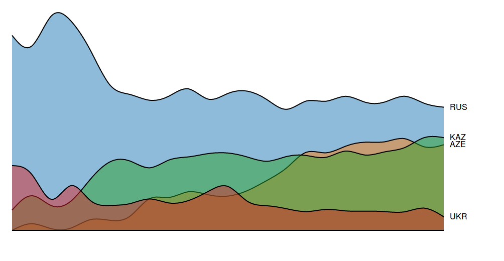
I felt like these templates weren’t designed to handle all the ex-Soviet countries, so for the top visualization I hand picked 4 countries that I believed had the most influence. Here’s all of them together: