No. 135: MIES – Simulating an Insurance Market

MIES, which stands for miniature insurance economic simulator, is a model of the insurance industry. during the course of my actuarial studies, I’ve been introduced to various concepts such as pricing, reserving, capital management, and regulation. While each topic made sense within the scope of the paper in which it was discussed, I never had a tool that I could use to put all the concepts together to get a cohesive narrative on their aggregate impact on the economy – that is, not just the impact on my employer (or department), but upon the insureds, other insurers, the uninsured, and the government. This has been my long-running attempt at making this tool.

I thought about making this many years ago, but soon discovered that I would need quite a lot of working experience as well as knowledge of various technologies. One thing I wanted to do was to represent each entity in the insurance sector as a class in object-oriented programming, which languages like R weren’t well-suited for. However, I’ve gotten the chance to use a lot of Python over the last few months and felt confident to put together my first self-sustaining simulation – as in, a simulation where policy issuance, pricing, and claims handling would happen in a self-sustaining cycle. This is what I’ll discuss today. As I continue to comb through literature and learn additional skills, I’ll gradually incorporate new aspects of the insurance industry into the model and relax assumptions to make things more realistic.

I’ve also developed the early versions of a few useful methods that were inspired by the slow-running processes I’ve often encountered on the job. For example, the function in_force() lets me, within a single line of code, return the entire in-force book for a business on any date. Believe it or not, what sounds like a straightforward request can take many days or even require a multi-month project at a real insurance company if the backend infrastructure is not built appropriately (in this particular scenario it’s not that writing the function is hard, but moreso dealing with something like a collection of incompatible databases left over from a long string of mergers and acquisitions – I hope other actuaries sympathize with me here). While I’ve applied this method on a highly simplified database, I just hope it gives some amount of motivation for anyone reading on what may be possible, if they’ve ever encountered a similar slow-running process at their own job.

Project Structure

As of today, the project contains four core modules that interact with each other to drive the simulations.

1. schema.py

Contains the ORM equivalent of the data definition language used to create the underling SQLite tables and define their relationships.

2. parameters.py

Contains the population characteristics from which the random variable parameters are derived.

3. entities.py

Contains the OOP representations of players in the insurance market, i.e., insurers, brokers, and customers.

4. simulation.py

Used to run the simulation, drawing objects from the other three modules.

Database Schema – SQLAlchemy/SQLite

The current database consists of a SQLite file. While I had previously mentioned that I would eventually like to have MIES running on postgres, using SQLite has made it easier for me to pursue rapid prototyping of various schemas without the cumbersome configuration process that comes with the postgres installation or other production-grade database management systems. SQLite does come with its disadvantages – for instance, it’s not quite as good with concurrency control or authorization in a multi-user environment.

One tool that I have been using to define and interact with the database file is SQLAlchemy, an object-relational mapper between Python and SQL. SQLAlchemy allows me to define and query the underlying MIES database without having to write any SQL. An object relational mapping is a framework used to reconcile a problem known as the object-relational impedance mismatch. The relational database model strives to achieve what’s known as program-data independence, that is, changes in the underlying data should not force changes in the software that depend on that data. On the other hand, in object-oriented programming languages like Python, data and the programs that manipulate that data are intricately linked, so trying to use SQL and Python together tends to break that independence. Therefore, an ORM tool like SQLAlchemy inserts a layer between the conflicting paradigms so as to minimize the disruption to the programs whenever the data change. Should the data change, you could update the mapping instead of having to update all the Python programs that depend on the data.

I have read varying opinions on the use of ORMs, but I have found writing embedded SQL queries, whether in R or Python, to be quite cumbersome, so I’ve decided to give SQLAlchemy a shot to see if I’d be more comfortable manipulating database tables as Python classes. I’ve liked it so far, although the learning curve can be steep, and more effort is required upfront to carefully define the schema and the relationships within it before you can query it with the ORM.

The database currently consists of a single SQLite file representing the entire insurance market. Once I learn how to implement multiple schemas and sessions within the simulation, it is my intention to split it up into multiple databases so that each entity (environment, brokers, insurers, etc.) receives its own database, which is closer to what you’d see in the real world. However, I’ve programmed the insurers in such a way that they cannot access each other’s data and can only build predictive models using their own book, so we should be okay for the limited applications that I’ve introduced in this early version.

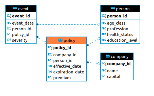
The following image shows the current ER diagram of the environment, consisting of four tables:

1. person

Represents the population and personal characteristics of the potential insureds.

2. company

Represents the insurance companies involved in the marketplace.

3. policy

Represents the policies written in the market. Each company can only access its own insureds.

4. event

Represents fortuitous events that can happen to people.

Person

While these tables can be created with a variety of tools, such as SQL data definition language (DDL), or ER diagramming software (for those preferring a GUI), SQLAlchemy lets us create them entirely in Python. Below, the person table is represented by the Person class, within which we specify its columns and relationships with other tables:

Each person in the market is identified by the unique identifier person_id, and are characterized by their age, profession, health status, and education level, which are dynamically generated for each simulation. This table has two relationships, one to the policy table, and another to the event table.

Policy

The policy table contains information for each policy, such as effective date, expiration date, premium, and company. This is the central table in the database, linking people, company, and insured events together:

Event

The event table contains fortuitous, financially damaging events that may happen to people. For this simulation, each event and person is insured, so there is no distinction between a claim and an event. Future simulations will relax those assumptions as not all risks are insured in the real world:

Company

The final table in the database contains company information. So far, the only important column is the identifier, which the company can use to determine a pricing model. You’ll see a definition for starting capital which will be used in future simulations to model profitability and return on capital, but for now it is unused:

If you look at the actual schema file in the GitHub repository, you’ll notice there’ also a table for claims. This has no use at the moment, but will in future versions once I start to differentiate between events and claims.

Simulation Parameters

One of the goals I prioritized for this version was to get a self-sustaining simulation running, which meant I made many simplifying assumptions to reduce the complexity of technical things I had to learn (such as multi-processing, multiple sessions, concurrency, time-based mathematics, etc.). These include:

1. Each iteration of the simulation begins on the last day of a calendar year.
2. All policies are effective on the following day, last for one year, and expire on the day of the next iteration.
3. All events happen on the first day policies become effective.
4. All events are covered, and are reported and paid immediately. There is no loss development.
5. Companies do not go bankrupt, and can exist indefinitely.
6. Each company can only develop pricing models on the business they have written.
7. During renewals, each person will simply choose the insurer that offers the lowest premium.
8. There are no policy expenses.

There are more assumptions, but these are the most obvious ones that I could think of. The parameters module in the repository contains values attached to each person’s characteristics, such as age class, stored in dictionaries. There is nothing particularly special about these values other than that they lead to five- to six-figure claim amounts, which are common in insurance. These values are used to generate parameters for the probability distributions that are used to generate event losses. These distributions are Poisson for event frequency and gamma for loss value:

You’ll see at the bottom of this file there are two functions, get_poisson_lambda() and get_gamma_scale(), these are used to generate the respective Poisson lambda and Gamma scale parameters on each iteration of the simulation, for each person.

Entities

Generating Insureds – Environment Class

The entities module contains class definitions for each entity in the simulation, beginning with the environment class:

The environment class is used to generate a underlying population of potential insureds, via the method make_population(). I use the word ‘potential’ since I would eventually like to model the availability of insurance, in which not all people will become insureds. However, each person in this simulation will become an insured, so for today’s purposes we can use the terms ‘person’ and ‘insured’ interchangeably.

This class is also used to generate fortuitous events that may happen to people. This is done via the smite() method, which for each person takes one draw from their respective Poisson frequency distribution and, for those persons experiencing an event(s), one or more draws from the gamma to simulate loss severity. The events that are generated via smite() are then stored in the event table.

The class also comes with a method called annihilate(), which is used to clean up the environment and remove the database prior to code distribution.

Placing Business – Broker Class

The broker class represents the insurance marketplace. The current version of the simulation has one broker, which serves as an intermediary between people and insurance companies to place business:

Within this class, the identify_free_business() method combs through the person table to identify any people who are either uninsured or have an expiring policy.

Once free business is assigned, the broker will then use the place_business() method to assign free business to insurers. In the initial pricing, during which all people are uninsured and each insurer offers the same initial premium, people are randomly allocated to each insured. On subsequent renewal pricings, each insurer will use their claim data to generate a pricing model, and the broker assigns person to the insurer with the lowest offered premium.

Pricing Business – Insurer Class

The insurer class represents the insurance company:

This class comes with a method called price_book(), which examines its historical book of business and loss experience to generate a pricing algorithm via GLM (Generalized Linear Model). Insurers are unaware of the true loss distribution of the underlying population, and thus must approximate it with a model. Here we use Tweedie distribution to generate a pure premium model for simplicity, an approach often taken under resource constraints (rather than building separate frequency and severity models). This method can accept any combination of response and set of independent variables. The model produced from this method will be attached to the insurer, which the broker can then use to price free business.

The Insurer class also comes with two methods to assist with analyzing model results: get_book() and in_force(), which returns the insurer’s historical book of business to date and in-force business, respectively.

Market Simulation – Two Companies

With the basic libraries defined, we’re now ready to run the simulation. In this scenario, we create a population of 1000 insureds, over which two insurers (Company 1 and Company 2) compete for business. One of them has a better pricing algorithm than the other, and we run the model over 100 underwriting periods to see how the market share changes between them.

Environment Setup

We start by importing the relevant modules for date manipulation, SQLAlchemy, and the MIES entity classes. The following code will import the object-relational mapping we defined earlier and use it to create a SQLite database, called MIES_Lite:

We next define the participants in the market, an environment object, which we’ll call ahura. We’ll call ahura’s make_population() method to create a market of 1000 people:

Next, three corporate entities, one broker named rayon and two insurance companies:

We now outline the strategy pursued by each firm. Company 1 will have the more refined pricing algorithm, using all four determinants of loss: age class, profession, health status, and education level. Company 2 uses a less refined strategy with only 1 rating variable, age class. We assume that each insured has the same exposure, so getting the pure premium is the same as dividing the sum of the losses for each insured by 1 (the severity below does actually represent a sum, which was obtained by a group by):

With the simulation set up the way it is, we should expect Company 2 to lose market share to Company 1. This is a well known phenomenon called adverse selection, and is a good candidate to test the early versions of MIES. Should something unexpected happen, such as Company 2 dominating the market on all simulations, we’ll know quickly whether something is wrong with model and if it needs to be fixed (this indeed happened while I was writing the modules).

Placing Business

The following loop defines the simulation, which will run 100 pricing periods. We’ll go through it one step at a time:

On the first iteration, everyone in the population is uninsured. Each company offers the same initial premium, 4000 as a prior estimate for each risk, therefore our broker rayon will make a random assignment of each person to the two companies:

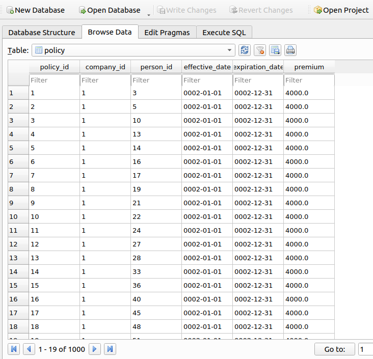
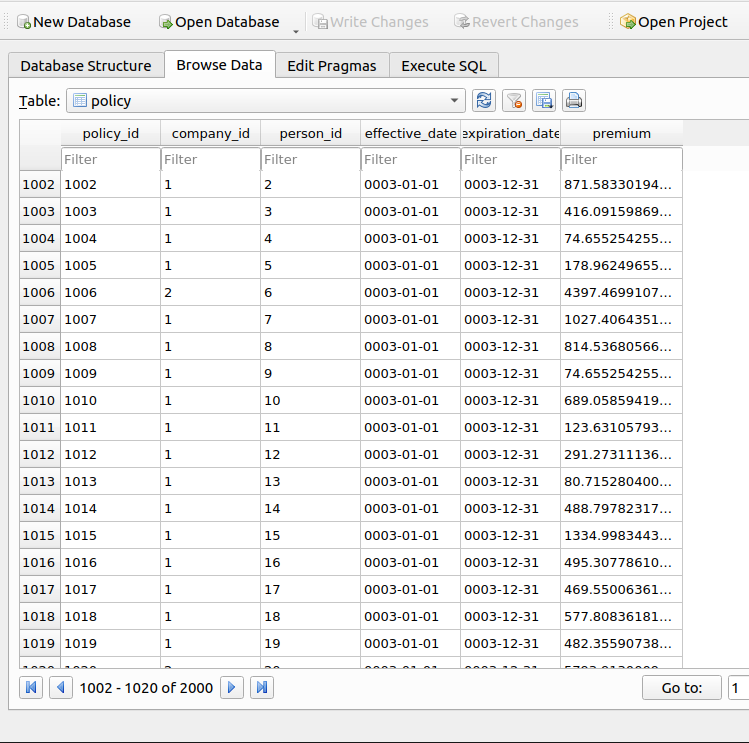
The following sample shows what the policy table looks like at this point in time:

Generating Claims

Now that the policies are allocated and written, we call ahura’s smite() method to wreak havoc upon the population, the day they begin coverage:

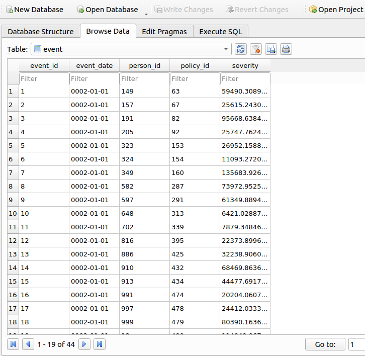
If we want to know what losses were generated, we can query the Event table in the database:

Repricing Business

Now that each insurer has claims experience, they now need to examine their books of business to recalibrate their premiums. We now call each insurer’s price_book() method to build a GLM from their data:

We then increment the date by one calendar year for the next iteration and save some results that we’ll use later for plotting:

Loop

The simulation repeats for 99 more periods. With each period, each company reprices its book based on the new claims data they acquire, and sends quotes to any customers looking to get insurance at their next renewal, including to the competing firm. The broker then assigns insureds to new customers depending on which insurer offers the lowest premium. Claims are then generated again and the cycle repeats. Here’s what the policies look like in the 2nd period, you can see that the premiums have been updated (from the original 4000) to reflect known information about the risk of each insured:

Evaluating Results

After 100 underwriting periods, we can clearly see adverse selection at work. Company 1, with a more refined pricing strategy captures the majority of the market over the simulation time horizon. There’s a brief period where Company 2 wins, but Company 1 has the better long term strategy:

Is adverse selection really happening? If so, we ought to see the average premium charged by Company 2 increase over time as the percentage of risky business in their book slowly increases over time. This is indeed the case:

Scalability – Four Firms (and Beyond)

MIES is designed to accept an arbitrary number of insureds, insurers, and pricing models. Let’s add two more insurers with different pricing strategies to see what happens:

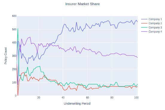
Both companies 3 and 4 have more refined strategies than company 2, but not as refined as company 1, so we’d expect their performance to be somewhere in between companies 1 and 2. After running the simulation, again, that’s what happens:

Interestingly, Company 4 outperformed Company 1 with respect to market share in the first 20 years or so. That’s a long time to be ahead with an inferior pricing formula, so that raises further questions – can a company lose even if they do things right? If so, could there, or should there be anything done about it? Or is Company 4 really winning? Just because they have a larger market share, are they writing it profitably? How does their mix of business look?

Further Improvements

I’ve got a long ways to go as far as adding features to MIES and making it more realistic. In reality, I’ll probably never stop working on it. Some ideas I have are:

1. Breaking up the database by participating entity
2. Relaxing time assumptions for claims and differentiating occurrence, report, payment, and settlement dates
3. Introducing loss development
4. Introducing policy limits and deductibles
5. Introducing reinsurance
6. Introducing policy expenses

And many more. If you’re interested in taking a look at the repository, it’s on my GitHub.