No. 92: Vector Addition in SAGE

Today I’d like to introduce you to some simple examples of vector addition in SAGE. I have been reading Lang’s introductory text to linear algebra, the first chapter of which covers properties of vectors.

SAGE can be used alongside Lang’s text as a gentle introduction to computer algebra systems. In my experience, I’ve found that bridging the gap between computer and paper mathematics can be intimidating, especially if a mathematics student doesn’t have a background in computer programming.

I’ve previously outlined why I think SAGE is an ideal educational tool, but to rehash it’s mainly because SAGE is open source and it uses Python as the language to execute commands. The open source nature of the software allows the student to examine what exactly is going on behind the user interface, and Python is a high-level programming language that lets the student execute commands right away without getting bogged down with low-level details like computer memory management.

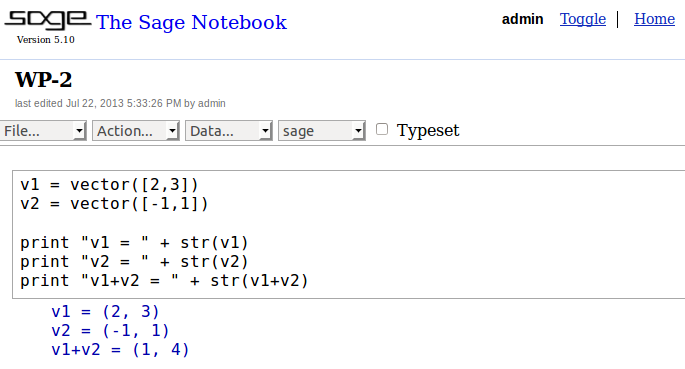
To get started, I’ll declare and print two vectors in SAGE, v1 and v2:

The first two lines in the above example declare the two vectors as variables, and the last three lines print v1, v2, and their sum in the output. Declaration of variables and the print function should be familiar to Python users.

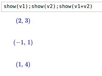
We can also use SAGE to display the vectors in prettyprint, which means to display the vectors in a manner similar to what you’d see in a publication:

Furthermore the latex() function outputs the LaTeX code – which is what you’d use to typeset such a publication:

In this case you would type \left(2,\,3\right) in your LaTeX editor.

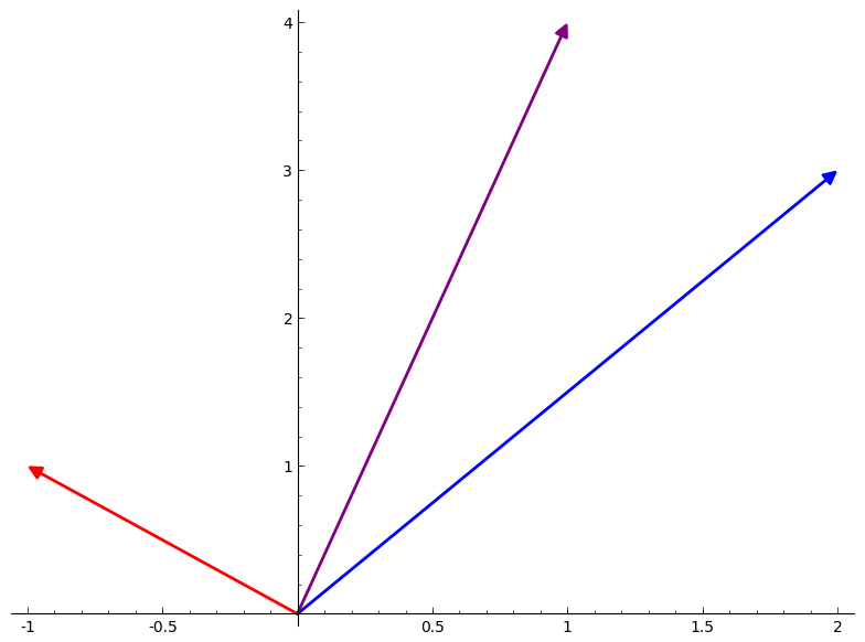
In the following diagram, you can see that each vector can be represented as a point on a two-dimensional plane. v1 and v2 are represented in blue and red, respectively, and their sum, v1+v2, in purple:

[code language=”python”]
show(plot(v1,color=”blue”)+plot(v2,color=”red”)+plot(v1+v2,color=”purple”))
[/code]

We can now use SAGE’s plotting capabilities to depict the Parallelogram Rule for vector addition, which states that the sum of two vectors can be represented as the fourth vertex of the parallelogram whose other three vertices are the two component vectors and the origin:

[code language=”python”]
l1=line([[1,4],[2,3]],linestyle=”–“,color=”black”)
l2=line([[-1,1],[1,4]],linestyle=”–“,color=”black”)
show(plot(v1,color=”blue”)+plot(v2,color=”red”)+plot(v1+v2,color=”purple”)+plot(l1)+plot(l2))
[/code]

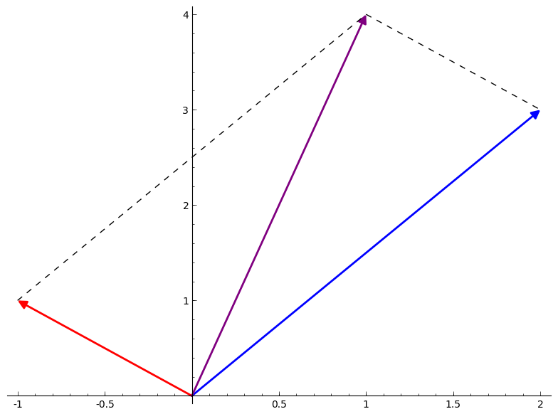Here, I have declared two additional variables as dashed line segments, and added them to the plot to complete the parallelogram.

SAGE also lets you declare and plot polygons. In the example below I have declared two polygons, p1 and p2, and shaded them in violet blue and violet red, respectively:

[code language=”python”]
p1 = polygon([(0,0),(1,4),(2,3)],rgbcolor=(138/256,43/256,226/256))
p2 = polygon([(-1,1),(0,0),(1,4)],rgbcolor=(219/256,112/256,147/256))
show(plot(v1,color=”blue”)+plot(v2,color=”red”)+plot(v1+v2,color=”purple”)+plot(l1)+plot(l2)+plot(p1)+plot(p2))
[/code]

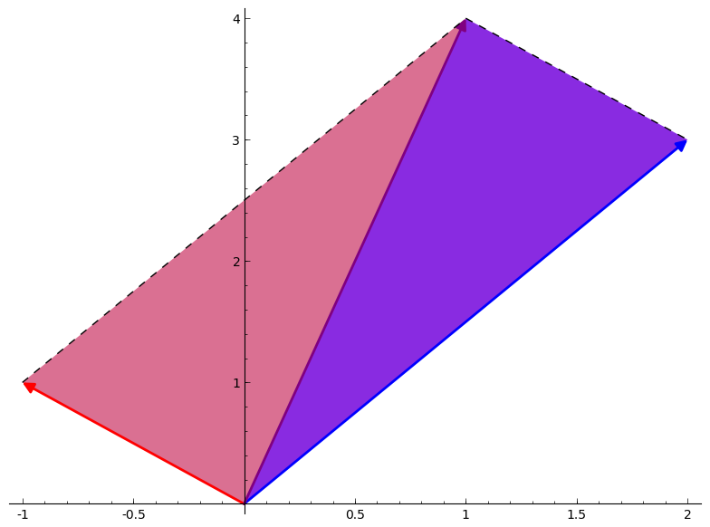As you can see, the parallelogram can be depicted as two triangles of equal size.

That’s it for today. I’ll soon follow up with another post on vector multiplication, and maybe some more properties such as equivalence and parallelism.