Gene Dan's Blog

No. 118: 25 Days of Network Theory – Day 1 – Introduction

5 July, 2017 11:14 AM / Leave a Comment / Gene Dan

I’ve decided to dedicate this month to the study of network theory. For the past few years, I’ve been intrigued not only by the theory’s simplicity – that a graph is simply a collection of nodes and edges, but also its ability to answer seemingly complex and qualitative questions regarding society (both human and nonhuman) in general, such as:

Who are the most influential members of society?
What are the most natural subdivisions for identifying communities within a population of people?
How can we construct a transportation system that optimizes traffic flow and minimizes traffic jams?
How can small disruptions spread through a network to cause financial crises?
How can we quantify consensus?
How are social norms and reputational effects enforced?
How quickly can a disease spread throughout a community?

…and so on.

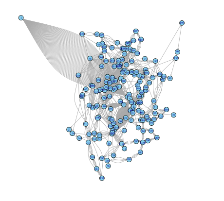
At first glance, the above graph may not look like anything special – but there is indeed something very special about it. This network represents co-occurrences between characters in Victor Hugo’s Les Miserables. After we add some labels to identify the characters, and adjust the size of the nodes and labels to reflect the degree (that is, the number of edges a node participates in), the graph becomes more meaningful in that you can immediately identify the most important characters to the plot:

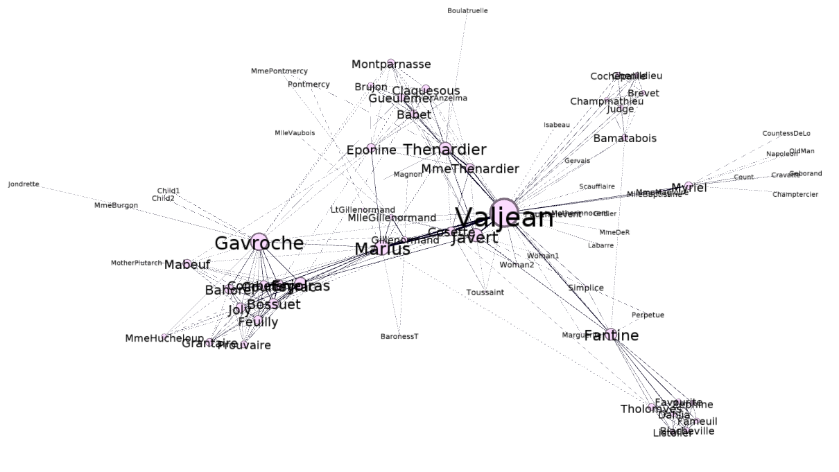
You can see that the largest node is represents Jean Valjean, the main protagonist of the story. This means that, at least according to degree, Jean Valjean is the most important person in the novel. However, there are several other quantitative measures of influence, and we will later see that Jean Valjean may not be the most influential character in the book, at least according to those other measures.

For this course, I’ll be reading Estrada and Knight’s, A First Course in Network Theory, and I’ll be reading 10 pages per day and applying what I learned there to the Les Miserables network.

There wasn’t much to the first ten pages other than to introduce the history of graph theory (there was a section on the Seven Bridges of Königsberg). So, I’ve used this opportunity to introduce what tools I’ll be using for the course of study. There’s gephi, a graph visualization program, igraph, a package that I’ll be using to perform more quantitative analyses on this network in R, and the Les Miserables network dataset itself.

Posted in: Mathematics

No. 117: Amino Acid Structural Formulas with Chemfig (Nonpolar Side Chains)

28 March, 2017 7:46 PM / 1 Comment / Gene Dan

$\LaTeX$ can do some pretty neat things. While it’s mostly known for typesetting mathematical notation, it can also be used to render structural formulas via the chemfig package, which makes it useful in the electronic communication of chemistry concepts – for example, it would allow two chemists located in different countries to chat over a message board, easing collaboration.

I’ll demonstrate some of the capabilities of chemfig by rendering the structural formulas of amino acids – 20 distinct molecules that serve as the building blocks of proteins – that is, the basis of cellular activity. Below are structural formulas for 9 of these, the ones with nonpolar side chains (this means that the side chains are hydrophobic, and do not have an affinity for water).

Amino Acid Structure
The basic structure of an amino acid consists of an asymmetric carbon bonded to four components – a hydrogen atom, an amino group, a carboxyl group, and an R-group. The amino group can act as a base, accepting a hydrogen ion. The carboxyl group can act as an acid (hence the name, amino acid), donating a hydrogen ion. The R-group is what gives a particular amino acid its identity (that is, whether a particular amino acid is glycine, tryptophan, etc.). It is unique for each type of amino acid and dictates its behavior. The amino group of one amino acid can bond with the carboxyl group of another amino acid, forming a peptide bond. When several amino acids are linked in a chain, they form a polypeptide – and one or more polypeptides together form a protein molecule.

Rendered by QuickLaTeX.com

This basic structure serves as a template for each of the amino acids below. The amino and carboxyl groups, together with the asymetric carbon and lower hydrogen atom, form the amino acid’s contribution to the polypeptide backbone. These are highlighted in blue. The R-group, distinct for each amino acid, is highlighted in red.

Notice that each of the code samples below contains a repeating pattern – \chemfig renders the structural formula of the amino acid. \chemmove draws the boxes that highlight the backbone and R-groups.

\chemfig{
C(-[:180]@{AR}N(-[:135]H)(-[:225]@{AL}H))(-[:0]@{CL}C(=[:45]@{CR}O)(-[:315]OH))(-[:90]@{R}R)(-[:270]H)
}

\chemmove{
  \draw[
    fill=purple,
    draw=purple,
    fill opacity=.2,
    rounded corners=2pt
  ]
    ([xshift=-3pt,yshift=-3pt]R.south west) 
    rectangle
    ([xshift=4pt,yshift=3pt]R.north east)   node[xshift=0pt,yshift=5pt,above,opacity=1,orientation]{R Group (Side Chain)};
}

\chemmove{
  \draw[
    fill=cyan,
    draw=cyan,
    fill opacity=.1,
    rounded corners=2pt
  ]
    ([xshift=-6pt,yshift=-15pt]AL.south west) node[xshift=15pt,yshift=-6pt,below,opacity=1,orientation]{Amino Group}
    rectangle
    ([xshift=3pt,yshift=35pt]AR.north east)
 ;
}

\chemmove{
  \draw[
    fill=cyan,
    draw=cyan,
    fill opacity=.1,
    rounded corners=2pt
  ]
    ([xshift=-3pt,yshift=-39pt]CL.south west) node[xshift=24pt,yshift=-6pt,below,opacity=1,orientation]{Carboxyl Group}
    rectangle
    ([xshift=12pt,yshift=12pt]CR.north east)
 ;
}

\chemfig{

C(-[:180]@{AR}N(-[:135]H)(-[:225]@{AL}H))(-[:0]@{CL}C(=[:45]@{CR}O)(-[:315]OH))(-[:90]@{R}R)(-[:270]H)

}

\chemmove{

\draw[

fill=purple,

draw=purple,

fill opacity=.2,

rounded corners=2pt

]

([xshift=-3pt,yshift=-3pt]R.south west)

rectangle

([xshift=4pt,yshift=3pt]R.north east) node[xshift=0pt,yshift=5pt,above,opacity=1,orientation]{R Group (Side Chain)};

}

\chemmove{

\draw[

fill=cyan,

draw=cyan,

fill opacity=.1,

rounded corners=2pt

]

([xshift=-6pt,yshift=-15pt]AL.south west) node[xshift=15pt,yshift=-6pt,below,opacity=1,orientation]{Amino Group}

rectangle

([xshift=3pt,yshift=35pt]AR.north east)

;

}

\chemmove{

\draw[

fill=cyan,

draw=cyan,

fill opacity=.1,

rounded corners=2pt

]

([xshift=-3pt,yshift=-39pt]CL.south west) node[xshift=24pt,yshift=-6pt,below,opacity=1,orientation]{Carboxyl Group}

rectangle

([xshift=12pt,yshift=12pt]CR.north east)

;

}

Glycine

For glycine, the R-group is a single hydrogen atom.

Rendered by QuickLaTeX.com

\chemfig{
C(-[:0]C(-[:0]@{C}O^{-})(=[:270]O))
(-[:270]H)(-[:180]H_3N^{+}(-[:270,1,,,draw=none]@{A}))
(-[:90]@{R}H)
}

\chemmove{
  \draw[
    fill=purple,
    draw=purple,
    fill opacity=.2,
    rounded corners=2pt
  ]
    ([xshift=-3pt,yshift=-3pt]R.south west)
    rectangle
    ([xshift=4pt,yshift=3pt]R.north east) ;
}

\chemmove{
  \draw[
    fill=cyan,
    draw=cyan,
    fill opacity=.1,
    rounded corners=2pt
  ]
    ([xshift=-9pt,yshift=-7pt]A.south west)
    rectangle
    ([xshift=3pt,yshift=5pt]C.north east)
 ;
}

\chemfig{

C(-[:0]C(-[:0]@{C}O^{-})(=[:270]O))

(-[:270]H)(-[:180]H_3N^{+}(-[:270,1,,,draw=none]@{A}))

(-[:90]@{R}H)

}

\chemmove{

\draw[

fill=purple,

draw=purple,

fill opacity=.2,

rounded corners=2pt

]

([xshift=-3pt,yshift=-3pt]R.south west)

rectangle

([xshift=4pt,yshift=3pt]R.north east) ;

}

\chemmove{

\draw[

fill=cyan,

draw=cyan,

fill opacity=.1,

rounded corners=2pt

]

([xshift=-9pt,yshift=-7pt]A.south west)

rectangle

([xshift=3pt,yshift=5pt]C.north east)

;

}

Alanine

The R-group for alanine is a little more complex than that of glycine, consisting of a methyl group instead of a hydrogen atom.

Rendered by QuickLaTeX.com

\chemfig{
C(-[:0]C(-[:0]@{C}O^{-})(=[:270]O))
(-[:270]H)(-[:180]H_3N^{+}(-[:270,1,,,draw=none]@{A}))
(-[:90]@{RL}CH_{3})
}

\chemmove{
  \draw[
    fill=purple,
    draw=purple,
    fill opacity=.2,
    rounded corners=2pt
  ]
    ([xshift=-3pt,yshift=-5pt]RL.south west)
    rectangle
    ([xshift=16pt,yshift=3pt]RL.north east) ;
}

\chemmove{
  \draw[
    fill=cyan,
    draw=cyan,
    fill opacity=.1,
    rounded corners=2pt
  ]
    ([xshift=-9pt,yshift=-7pt]A.south west)
    rectangle
    ([xshift=3pt,yshift=5pt]C.north east)
 ;
}

\chemfig{

C(-[:0]C(-[:0]@{C}O^{-})(=[:270]O))

(-[:270]H)(-[:180]H_3N^{+}(-[:270,1,,,draw=none]@{A}))

(-[:90]@{RL}CH_{3})

}

\chemmove{

\draw[

fill=purple,

draw=purple,

fill opacity=.2,

rounded corners=2pt

]

([xshift=-3pt,yshift=-5pt]RL.south west)

rectangle

([xshift=16pt,yshift=3pt]RL.north east) ;

}

\chemmove{

\draw[

fill=cyan,

draw=cyan,

fill opacity=.1,

rounded corners=2pt

]

([xshift=-9pt,yshift=-7pt]A.south west)

rectangle

([xshift=3pt,yshift=5pt]C.north east)

;

}

Valine

Rendered by QuickLaTeX.com

\chemfig{
C(-[:0]C(-[:0]@{C}O^{-})(=[:270]O))
(-[:270]H)(-[:180]H_3N^{+}(-[:270,1,,,draw=none]@{A}))
(-[:90]CH(-[:135]CH_{3})(-[:45]@{RR}CH_{3})(-[:180,1,,,draw=none]@{RL}))
}

\chemmove{
  \draw[
    fill=purple,
    draw=purple,
    fill opacity=.2,
    rounded corners=2pt
  ]
    ([xshift=-9pt,yshift=-9pt]RL.south west)
    rectangle
    ([xshift=15pt,yshift=6pt]RR.north east) ;
}

\chemmove{
  \draw[
    fill=cyan,
    draw=cyan,
    fill opacity=.1,
    rounded corners=2pt
  ]
    ([xshift=-9pt,yshift=-7pt]A.south west)
    rectangle
    ([xshift=3pt,yshift=5pt]C.north east)
 ;
}

\chemfig{

C(-[:0]C(-[:0]@{C}O^{-})(=[:270]O))

(-[:270]H)(-[:180]H_3N^{+}(-[:270,1,,,draw=none]@{A}))

(-[:90]CH(-[:135]CH_{3})(-[:45]@{RR}CH_{3})(-[:180,1,,,draw=none]@{RL}))

}

\chemmove{

\draw[

fill=purple,

draw=purple,

fill opacity=.2,

rounded corners=2pt

]

([xshift=-9pt,yshift=-9pt]RL.south west)

rectangle

([xshift=15pt,yshift=6pt]RR.north east) ;

}

\chemmove{

\draw[

fill=cyan,

draw=cyan,

fill opacity=.1,

rounded corners=2pt

]

([xshift=-9pt,yshift=-7pt]A.south west)

rectangle

([xshift=3pt,yshift=5pt]C.north east)

;

}

Leucine

Rendered by QuickLaTeX.com

\chemfig{
C(-[:0]C(-[:0]@{C}O^{-})(=[:270]O))
(-[:270]H)(-[:180]H_3N^{+}(-[:270,1,,,draw=none]@{A}))
(-[:90]CH_{2}((-[:90]CH(-[:135]CH_{3})(-[:45]@{RR}CH_{3})))(-[:180,1,,,draw=none]@{RL}))
}

\chemmove{
  \draw[
    fill=purple,
    draw=purple,
    fill opacity=.2,
    rounded corners=2pt
  ]
    ([xshift=-9pt,yshift=-9pt]RL.south west)
    rectangle
    ([xshift=15pt,yshift=9pt]RR.north east) ;
}

\chemmove{
  \draw[
    fill=cyan,
    draw=cyan,
    fill opacity=.1,
    rounded corners=2pt
  ]
    ([xshift=-9pt,yshift=-7pt]A.south west)
    rectangle
    ([xshift=3pt,yshift=5pt]C.north east)
 ;
}

\chemfig{

C(-[:0]C(-[:0]@{C}O^{-})(=[:270]O))

(-[:270]H)(-[:180]H_3N^{+}(-[:270,1,,,draw=none]@{A}))

(-[:90]CH_{2}((-[:90]CH(-[:135]CH_{3})(-[:45]@{RR}CH_{3})))(-[:180,1,,,draw=none]@{RL}))

}

\chemmove{

\draw[

fill=purple,

draw=purple,

fill opacity=.2,

rounded corners=2pt

]

([xshift=-9pt,yshift=-9pt]RL.south west)

rectangle

([xshift=15pt,yshift=9pt]RR.north east) ;

}

\chemmove{

\draw[

fill=cyan,

draw=cyan,

fill opacity=.1,

rounded corners=2pt

]

([xshift=-9pt,yshift=-7pt]A.south west)

rectangle

([xshift=3pt,yshift=5pt]C.north east)

;

}

Isoleucine

Rendered by QuickLaTeX.com

\chemfig{
C(-[:0]C(-[:0]@{C}O^{-})(=[:270]O))
(-[:270]H)(-[:180]H_3N^{+}(-[:270,1,,,draw=none]@{A}))
(-[:90]CH(-[:180]@{RL}H_3C)(-[:90]CH_{2}(-[:90]@{RR}CH_{3})))
}

\chemmove{
  \draw[
    fill=purple,
    draw=purple,
    fill opacity=.2,
    rounded corners=2pt
  ]
    ([xshift=-6pt,yshift=-9pt]RL.south west)
    rectangle
    ([xshift=18pt,yshift=9pt]RR.north east) ;
}

\chemmove{
  \draw[
    fill=cyan,
    draw=cyan,
    fill opacity=.1,
    rounded corners=2pt
  ]
    ([xshift=-9pt,yshift=-7pt]A.south west)
    rectangle
    ([xshift=3pt,yshift=5pt]C.north east)
 ;
}

\chemfig{

C(-[:0]C(-[:0]@{C}O^{-})(=[:270]O))

(-[:270]H)(-[:180]H_3N^{+}(-[:270,1,,,draw=none]@{A}))

(-[:90]CH(-[:180]@{RL}H_3C)(-[:90]CH_{2}(-[:90]@{RR}CH_{3})))

}

\chemmove{

\draw[

fill=purple,

draw=purple,

fill opacity=.2,

rounded corners=2pt

]

([xshift=-6pt,yshift=-9pt]RL.south west)

rectangle

([xshift=18pt,yshift=9pt]RR.north east) ;

}

\chemmove{

\draw[

fill=cyan,

draw=cyan,

fill opacity=.1,

rounded corners=2pt

]

([xshift=-9pt,yshift=-7pt]A.south west)

rectangle

([xshift=3pt,yshift=5pt]C.north east)

;

}

Methionine

Rendered by QuickLaTeX.com

\chemfig{
C(-[:0]C(-[:0]@{C}O^{-})(=[:270]O))
(-[:270]H)(-[:180]H_3N^{+}(-[:270,1,,,draw=none]@{A}))
(-[:90]@{RL}CH_{2}(-[:90]CH_{2}(-[:90]S(-[:90]@{RR}CH_{3}))))
}

\chemmove{
  \draw[
    fill=purple,
    draw=purple,
    fill opacity=.2,
    rounded corners=2pt
  ]
    ([xshift=-6pt,yshift=-9pt]RL.south west)
    rectangle
    ([xshift=18pt,yshift=9pt]RR.north east) ;
}

\chemmove{
  \draw[
    fill=cyan,
    draw=cyan,
    fill opacity=.1,
    rounded corners=2pt
  ]
    ([xshift=-9pt,yshift=-7pt]A.south west)
    rectangle
    ([xshift=3pt,yshift=5pt]C.north east)
 ;
}

\chemfig{

C(-[:0]C(-[:0]@{C}O^{-})(=[:270]O))

(-[:270]H)(-[:180]H_3N^{+}(-[:270,1,,,draw=none]@{A}))

(-[:90]@{RL}CH_{2}(-[:90]CH_{2}(-[:90]S(-[:90]@{RR}CH_{3}))))

}

\chemmove{

\draw[

fill=purple,

draw=purple,

fill opacity=.2,

rounded corners=2pt

]

([xshift=-6pt,yshift=-9pt]RL.south west)

rectangle

([xshift=18pt,yshift=9pt]RR.north east) ;

}

\chemmove{

\draw[

fill=cyan,

draw=cyan,

fill opacity=.1,

rounded corners=2pt

]

([xshift=-9pt,yshift=-7pt]A.south west)

rectangle

([xshift=3pt,yshift=5pt]C.north east)

;

}

Phenylalanine

Rendered by QuickLaTeX.com

\chemfig{
C(-[:0]C(-[:0]@{C}O^{-})(=[:270]O))
(-[:270]H)(-[:180]H_3N^{+}(-[:270,1,,,draw=none]@{A}))
(-[:90]@{RL}CH_{2}(-[:90]*6(-=-@{RR}=-=)))
}

\chemmove{
  \draw[
    fill=purple,
    draw=purple,
    fill opacity=.2,
    rounded corners=2pt
  ]
    ([xshift=-33pt,yshift=-9pt]RL.south west)
    rectangle
    ([xshift=36pt,yshift=6pt]RR.north east) ;
}

\chemmove{
  \draw[
    fill=cyan,
    draw=cyan,
    fill opacity=.1,
    rounded corners=2pt
  ]
    ([xshift=-9pt,yshift=-7pt]A.south west)
    rectangle
    ([xshift=3pt,yshift=5pt]C.north east)
 ;
}

\chemfig{

C(-[:0]C(-[:0]@{C}O^{-})(=[:270]O))

(-[:270]H)(-[:180]H_3N^{+}(-[:270,1,,,draw=none]@{A}))

(-[:90]@{RL}CH_{2}(-[:90]*6(-=-@{RR}=-=)))

}

\chemmove{

\draw[

fill=purple,

draw=purple,

fill opacity=.2,

rounded corners=2pt

]

([xshift=-33pt,yshift=-9pt]RL.south west)

rectangle

([xshift=36pt,yshift=6pt]RR.north east) ;

}

\chemmove{

\draw[

fill=cyan,

draw=cyan,

fill opacity=.1,

rounded corners=2pt

]

([xshift=-9pt,yshift=-7pt]A.south west)

rectangle

([xshift=3pt,yshift=5pt]C.north east)

;

}

Tryptophan

This was definitely the hardest of the amino acids to draw so far. It took multiple attempts to get the ring structure correct. I also had a problem rendering the full image (the top was being cropped off). I actually have an invisible structure embedded in the page code that serves as a workaround to getting the full image rendered.

Rendered by QuickLaTeX.com

\chemfig{
C(-[:0]C(-[:0]@{C}O^{-})(=[:270]O))
(-[:270]H)(-[:180]H_3N^{+}(-[:270,1,,,draw=none]@{A}))
(-[:90]@{RL}CH_{2}(-[:90]?(*6([::-30]=-NH-(*6(--@{RR}----))=?))))
}

\chemmove{
  \draw[
    fill=purple,
    draw=purple,
    fill opacity=.2,
    rounded corners=2pt
  ]
    ([xshift=-33pt,yshift=-9pt]RL.south west)
    rectangle
    ([xshift=36pt,yshift=6pt]RR.north east) ;
}

\chemmove{
  \draw[
    fill=cyan,
    draw=cyan,
    fill opacity=.1,
    rounded corners=2pt
  ]
    ([xshift=-9pt,yshift=-7pt]A.south west)
    rectangle
    ([xshift=3pt,yshift=5pt]C.north east)
 ;
}
\chemfig{
-[:90,1,,,draw=none](-[:90,1,,,draw=none])
}

\chemfig{

C(-[:0]C(-[:0]@{C}O^{-})(=[:270]O))

(-[:270]H)(-[:180]H_3N^{+}(-[:270,1,,,draw=none]@{A}))

(-[:90]@{RL}CH_{2}(-[:90]?(*6([::-30]=-NH-(*6(--@{RR}----))=?))))

}

\chemmove{

\draw[

fill=purple,

draw=purple,

fill opacity=.2,

rounded corners=2pt

]

([xshift=-33pt,yshift=-9pt]RL.south west)

rectangle

([xshift=36pt,yshift=6pt]RR.north east) ;

}

\chemmove{

\draw[

fill=cyan,

draw=cyan,

fill opacity=.1,

rounded corners=2pt

]

([xshift=-9pt,yshift=-7pt]A.south west)

rectangle

([xshift=3pt,yshift=5pt]C.north east)

;

}

\chemfig{

-[:90,1,,,draw=none](-[:90,1,,,draw=none])

}

Proline

Rendered by QuickLaTeX.com

\chemfig{
C(-[:0]C(-[:0]@{C}O^{-})(=[:270]O))
(-[:270]H)(-[:180]H_3N^{+}(-[:270,1,,,draw=none]@{A})(-[:90]@{RL}H_{2}C?))
(-[:90]CH_{2}(-[:120]@{RR}CH_{2}?))
}

\chemmove{
  \draw[
    fill=purple,
    draw=purple,
    fill opacity=.2,
    rounded corners=2pt
  ]
    ([xshift=-3pt,yshift=-9pt]RL.south west)
    rectangle
    ([xshift=42pt,yshift=9pt]RR.north east) ;
}

\chemmove{
  \draw[
    fill=cyan,
    draw=cyan,
    fill opacity=.1,
    rounded corners=2pt
  ]
    ([xshift=-9pt,yshift=-7pt]A.south west)
    rectangle
    ([xshift=3pt,yshift=5pt]C.north east)
 ;
}

\chemfig{

C(-[:0]C(-[:0]@{C}O^{-})(=[:270]O))

(-[:270]H)(-[:180]H_3N^{+}(-[:270,1,,,draw=none]@{A})(-[:90]@{RL}H_{2}C?))

(-[:90]CH_{2}(-[:120]@{RR}CH_{2}?))

}

\chemmove{

\draw[

fill=purple,

draw=purple,

fill opacity=.2,

rounded corners=2pt

]

([xshift=-3pt,yshift=-9pt]RL.south west)

rectangle

([xshift=42pt,yshift=9pt]RR.north east) ;

}

\chemmove{

\draw[

fill=cyan,

draw=cyan,

fill opacity=.1,

rounded corners=2pt

]

([xshift=-9pt,yshift=-7pt]A.south west)

rectangle

([xshift=3pt,yshift=5pt]C.north east)

;

}

Posted in: Uncategorized / Tagged: acid, amino, chemfig, LaTeX, structural formula

No. 116: 70 Days of Linear Algebra (Day 9)

30 November, 2016 6:51 PM / Leave a Comment / Gene Dan

Section: 1.6 – Applications of Linear Systems

Linear systems can be used to model and solve problems concerning traffic flow. Consider for instance, the following set of intersections modeled by a graph:

The orchid nodes G, H, J, and K represent traffic inflows. The pink nodes E, F, and I represent traffic outflows. The blue nodes A, B, C, and D represent intersections. Each edge (the lines connecting the nodes – representing roads) is labeled with the traffic flow measured in cars per hour. For example, 500 cars travel from J to A each hour. Assuming that for each intersection (and for the network as a whole), that traffic inflow equals traffic outflow, one question arises regarding capacity – how much traffic should the roads x₁, x₂, x₃, x₄, and x₅ be designed to handle?

First, we need to determine traffic inflows and outflows for each intersection:

Intersection	Flow In	Flow Out
A	300 + 500	x₁ + x₂
B	x₂ + x₄	300 + x₃
C	400 + 100	x₄ + x₅
D	x₁ + x₅	600

In addition, we have the constraint that total network inflow (500 + 300 + 100 + 400) equal total network outflow (300 + x₃ + 600), so x₃ = 400.

We can use this information to represent the network as a system of linear equations and row reduce the corresponding augmented matrix to solve for the unknowns:

\[\begin{aligned} x_1+x_2&=800\\x_2-x_3+x_4&=300\\x_4+x_5&=500\\x_1+x_5&=600\\x_3&=400\end{aligned}\]

\[\left[\begin{array}{cccccc} 1 & 1 & 0 & 0 & 0 & 800 \\ 0 & 1 & -1 & 1 & 0 & 300 \\ 0 & 0 & 0 & 1 & 1 & 500 \\ 1 & 0 & 0 & 0 & 1 & 600 \\ 0 & 0 & 1 & 0 & 0 & 400 \\ \end{array}\right] \sim \left[\begin{array}{cccccc} 1 & 0 & 0 & 0 & 1 & 600 \\ 0 & 1 & 0 & 0 & -1 & 200 \\ 0 & 0 & 1 & 0 & 0 & 400 \\ 0 & 0 & 0 & 1 & 1 & 500 \\ 0 & 0 & 0 & 0 & 0 & 0 \end{array} \right] \]

Which leads us to the general solution:

\[\left\{\begin{aligned} x_1 & = 600 – x_5 \\ x_2 &=200+x_5 \\ x_3&=400\\x_4&=500-x_5\\x_5&\text{ is free} \end{aligned}\right.\]

Since x₅ is free, we have infinitely many solutions to the problem. Thus, in practice, how we actually design the roads would depend on how much traffic we anticipate for x₅.

Code used to create the graph

library(igraph)

edges <- c("B","E"
          ,"B","F"
          ,"A","B"
          ,"C","B"
          ,"G","C"
          ,"H","C"
          ,"C","D"
          ,"D","I"
          ,"J","A"
          ,"K","A"
          ,"A","D")

edge_labels <- c("300"
                ,"x3"
                ,"x2"
                ,"x4"
                ,"100"
                ,"400"
                ,"x5"
                ,"600"
                ,"500"
                ,"300"
                ,"x1")

cols <- c("skyblue"
          ,"pink"
          ,"pink"
          ,"skyblue"
          ,"skyblue"
          ,"orchid"
          ,"orchid"
          ,"skyblue"
          ,"pink"
          ,"orchid"
          ,"orchid")
traffic <- graph(x) %>% set_edge_attr("label",value=edge_labels)
traffic$label <- edge_labels
plot(traffic
    ,vertex.color=cols
    ,edge.arrow.size=.4
)

library(igraph)

edges <- c("B","E"

,"B","F"

,"A","B"

,"C","B"

,"G","C"

,"H","C"

,"C","D"

,"D","I"

,"J","A"

,"K","A"

,"A","D")

edge_labels <- c("300"

,"x3"

,"x2"

,"x4"

,"100"

,"400"

,"x5"

,"600"

,"500"

,"300"

,"x1")

cols <- c("skyblue"

,"pink"

,"skyblue"

,"orchid"

,"skyblue"

,"pink"

,"orchid"

,"orchid")

traffic <- graph(x) %>% set_edge_attr("label",value=edge_labels)

traffic$label <- edge_labels

plot(traffic

,vertex.color=cols

,edge.arrow.size=.4

)

Code used to solve the equations

library(pracma)
A = matrix(c(1,1,0,0,0,800
            ,0,1,-1,1,0,300
            ,0,0,0,1,1,500
            ,1,0,0,0,1,600
            ,0,0,1,0,0,400)
            ,nrow=5,ncol=6,byrow=TRUE)
rref(A)

library(pracma)

A = matrix(c(1,1,0,0,0,800

,0,1,-1,1,0,300

,0,0,0,1,1,500

,1,0,0,0,1,600

,0,0,1,0,0,400)

,nrow=5,ncol=6,byrow=TRUE)

rref(A)

Posted in: Mathematics / Tagged: 70 days of linear algebra

No. 115: The Collatz Conjecture

22 November, 2016 7:52 PM / Leave a Comment / Gene Dan

The Collatz Conjecture is a famous unsolved problem in mathematics. Given any positive integer, if that integer is even, divide it by two. If it’s odd, multiply it by three and then add 1. Keep repeating until you get 1. The conjecture claims that no matter what number you start with, you will always reach 1.

Is this the case? Nobody knows! But let’s try a few examples: 12, 7, and 9

12 -> 6 -> 3 -> 10 -> 5 -> 16 -> 8 -> 4 -> 2 -> 1
7 -> 22 -> 11 -> 34 -> 17 -> 52 -> 26 -> 13 -> 40 -> 20 -> 10 -> 5 -> 16 -> 8 -> 4 -> 2 -> 1
9 -> 28 -> 14 -> 7 -> … 8 -> 4 -> 2 -> 1

In all three cases, we get a chain of numbers that eventually leads to 1. In fact, we can try every integer up to 100 million and we will still end up with 1! Given that a counterexample hasn’t been found for extremely large numbers, many people believe the conjecture to be true. The reason why this problem is so famous is because it’s easy to understand, but hard to solve.

Given the example above, we can construct a directed graph that plots each successive step for all situations up to a specified integer. For example, when n = 50:

We can see that every chain leads to 1, which is why so many arrows point to node 1. I’ve created a visualization using R Shiny, and using the slider below, you can see how the graph changes as you change n. I could go on about R Shiny, which is an extremely useful package for visualizing mathematical concepts due to its interactive nature, but since I’m busy, I’ll have to save that for a later time.

The code is contained in 3 files, server.R, ui.r, and helpers.R.

server.R:

library(shiny)
library(igraph)
source("helpers.R")
shinyServer(function(input, output) {
  
  output$distPlot <- renderPlot({
    out.n <- input$n
    pairs <- c()
    for(i in 1:out.n)
    {
      curr <- i
      while(curr != 1)
      {
        if(curr %% 2 == 0)
        {
          nxt <- curr / 2
        }
        else
        {
          nxt <- 3 * curr + 1
        }
        pairs <- c(pairs,as.character(curr),as.character(nxt))
        curr <- nxt
      }
    }
    graph.directed <- graph(pairs)
    l <- layout.forceatlas2(graph.directed, iterations=100,plotstep=0)
    plot(graph.directed,layout=l, vertex.color="skyblue", vertex.size=6, edge.arrow.size=.2, vertex.label.cex=.5)
  })
  
})

library(shiny)

library(igraph)

source("helpers.R")

shinyServer(function(input, output) {

output$distPlot <- renderPlot({

out.n <- input$n

pairs <- c()

for(i in 1:out.n)

{

curr <- i

while(curr != 1)

{

if(curr %% 2 == 0)

{

nxt <- curr / 2

}

else

{

nxt <- 3 * curr + 1

}

pairs <- c(pairs,as.character(curr),as.character(nxt))

curr <- nxt

}

graph.directed <- graph(pairs)

l <- layout.forceatlas2(graph.directed, iterations=100,plotstep=0)

plot(graph.directed,layout=l, vertex.color="skyblue", vertex.size=6, edge.arrow.size=.2, vertex.label.cex=.5)

})

ui.r

library(shiny)

shinyUI(fluidPage(
  
  # Application title
  titlePanel("Collatz Conjecture"),
  withMathJax(
  HTML("Consider the following operation on an arbitrary positive integer:
            <ul>
            <li>If the number is even, divide it by two.</li>
            <li>If the number is odd, triple it and add one.</li>
            </ul></br>
  In modular arithmetic notation, define the function \\(f\\) as follows:</br>
$$f(x)= \\left\\{
\\begin{aligned}
     \\ n/2  &\\quad  \\text{if } n\\equiv0\\,(\\text{mod } 2)  \\\\
     \\ 3n+1 &\\quad  \\text{if } n\\equiv1\\,(\\text{mod } 2)  \\\\
     \\end{aligned}
     \\right.$$
  Now, form a sequence by performing this operation repeatedly, beginning with any positive integer, and taking the result at each step as the input at the next.
       In notation:
$$a_i=\\left\\{
       \\begin{aligned}
       \\ n          & \\quad \\text{for } i = 0 \\\\
       \\ f(a_{i-1}) & \\quad \\text{for i} >0 \\\\
       \\end{aligned}
       \\right.$$
  The Collatz conjecture is: <i>This process will eventually reach the number 1, regardless of which positive integer is chosen initially</i>.")),
  
  # Sidebar with a slider input for K 
  sidebarLayout(
    sidebarPanel(
       sliderInput("n",
                   "Directed graph for all sequences up to n:",
                   min = 2,
                   max = 100,
                   value = 50)
    ),
    
    
    mainPanel(
       plotOutput("distPlot",width="500px", height="500px")
    )
  )
))

library(shiny)

shinyUI(fluidPage(

# Application title

titlePanel("Collatz Conjecture"),

withMathJax(

HTML("Consider the following operation on an arbitrary positive integer:

<ul>

<li>If the number is even, divide it by two.</li>

<li>If the number is odd, triple it and add one.</li>

</ul></br>

In modular arithmetic notation, define the function \$f\$ as follows:</br>

$$f(x)= \\left\\{

\\begin{aligned}

\\ n/2 &\\quad \\text{if } n\\equiv0\\,(\\text{mod } 2) \\\\

\\ 3n+1 &\\quad \\text{if } n\\equiv1\\,(\\text{mod } 2) \\\\

\\end{aligned}

\\right.$$

Now, form a sequence by performing this operation repeatedly, beginning with any positive integer, and taking the result at each step as the input at the next.

In notation:

$$a_i=\\left\\{

\\begin{aligned}

\\ n & \\quad \\text{for } i = 0 \\\\

\\ f(a_{i-1}) & \\quad \\text{for i} >0 \\\\

\\end{aligned}

\\right.$$

The Collatz conjecture is: <i>This process will eventually reach the number 1, regardless of which positive integer is chosen initially</i>.")),

# Sidebar with a slider input for K

sidebarLayout(

sidebarPanel(

sliderInput("n",

"Directed graph for all sequences up to n:",

min = 2,

max = 100,

value = 50)

mainPanel(

plotOutput("distPlot",width="500px", height="500px")

)

))

The helpers.R file was taken here, and was used to apply the ForceAtlas 2 layout on the igraph package.

Posted in: Mathematics

No. 114: Visualizing the Blockchain

24 December, 2014 5:29 PM / Leave a Comment / Gene Dan

For those of you who don’t know what Bitcoin is, it’s a digital currency that’s been gaining attention over the last few years, mostly due to its obscure user base, popularity on the black market (although most bitcoin transactions are legal), and its exchange rate volatility versus the U.S. dollar.

I’ve been interested in Bitcoin for quite some time, since unlike cash transactions, all bitcoin transactions are recorded on a publicly available ledger called the Blockchain. Because the blockchain records all transactions that occur over the bitcoin network, it can be a valuable source of information, revealing interesting patterns about peer-to-peer monetary transactions that were previously unavailable under traditional currency, due to lack of available data.

I stumbled across some CSV files on the internet that contain parsed blockchain information available in a script-friendly format here. Using this dataset I wrote a script to extract the transactions from the first 500 bitcoin users:

#import dataset
#edges <- read.csv("user_edges.txt", header=FALSE)
#head(edges)

###subset first n users
lim <- 500
edges.sub <- edges[edges$V2 <= lim & edges $V3 <= lim & (edges$V2 != edges$V3), c("V2","V3")]
head(edges.sub,500)
sub.unique <- edges.sub[!duplicated(edges.sub),]
sub.unique$edgenum <- 1:nrow(sub.unique)
head(sub.unique)
sub.unique$edges <- paste('<edge id="', as.character(sub.unique$edgenum),'" source="', sub.unique$V2, '" target="',sub.unique$V3, '"/>',sep="")

###build nodes
nodes <- data.frame(id=sort(unique(c(sub.unique$V2,sub.unique$V3))))
nodes$nodestr <- paste('<node id="', as.character(nodes$id), '" label="',nodes$id, '"/>',sep="")
head(nodes)

### build metadata
gexfstr <- '<?xml version="1.0" encoding="UTF-8"?>
<gexf xmlns:viz="http:///www.gexf.net/1.1draft/viz" version="1.1" xmlns="http://www.gexf.net/1.1draft">
<meta lastmodifieddate="2010-03-03+23:44">
<creator>Gephi 0.7</creator>
</meta>
<graph defaultedgetype="undirected" idtype="string" type="static">'


### append nodes
gexfstr <- paste(gexfstr,'\n','<nodes count="',as.character(nrow(nodes)),'">\n',sep="")
fileConn<-file("output.gexf")
for(i in 1:nrow(nodes)){
  gexfstr <- paste(gexfstr,nodes$nodestr[i],"\n",sep="")}
gexfstr <- paste(gexfstr,'</nodes>\n','<edges count="',as.character(nrow(sub.unique)),'">\n',sep="")

### append edges and print to file
for(i in 1:nrow(sub.unique)){
  gexfstr <- paste(gexfstr,sub.unique$edges[i],"\n",sep="")}
gexfstr <- paste(gexfstr,'</edges>\n</graph>\n</gexf>',sep="")
writeLines(gexfstr, fileConn)
close(fileConn)

#import dataset

#edges <- read.csv("user_edges.txt", header=FALSE)

#head(edges)

###subset first n users

lim <- 500

edges.sub <- edges[edges$V2 <= lim & edges $V3 <= lim & (edges$V2 != edges$V3), c("V2","V3")]

head(edges.sub,500)

sub.unique <- edges.sub[!duplicated(edges.sub),]

sub.unique$edgenum <- 1:nrow(sub.unique)

head(sub.unique)

sub.unique$edges <- paste('<edge id="', as.character(sub.unique$edgenum),'" source="', sub.unique$V2, '" target="',sub.unique$V3, '"/>',sep="")

###build nodes

nodes <- data.frame(id=sort(unique(c(sub.unique$V2,sub.unique$V3))))

nodes$nodestr <- paste('<node id="', as.character(nodes$id), '" label="',nodes$id, '"/>',sep="")

head(nodes)

### build metadata

gexfstr <- '<?xml version="1.0" encoding="UTF-8"?>

<creator>Gephi 0.7</creator>

</meta>

<graph defaultedgetype="undirected" idtype="string" type="static">'

### append nodes

gexfstr <- paste(gexfstr,'\n','<nodes count="',as.character(nrow(nodes)),'">\n',sep="")

fileConn<-file("output.gexf")

for(i in 1:nrow(nodes)){

gexfstr <- paste(gexfstr,nodes$nodestr[i],"\n",sep="")}

gexfstr <- paste(gexfstr,'</nodes>\n','<edges count="',as.character(nrow(sub.unique)),'">\n',sep="")

### append edges and print to file

for(i in 1:nrow(sub.unique)){

gexfstr <- paste(gexfstr,sub.unique$edges[i],"\n",sep="")}

gexfstr <- paste(gexfstr,'</edges>\n</graph>\n</gexf>',sep="")

writeLines(gexfstr, fileConn)

close(fileConn)

I subsequently imported the output file into gephi to create a network visualization of the transactions. You can view the process in the video below.

https://www.youtube.com/watch?v=wjw0ksaRSO4&feature=youtu.be

The resulting graph:

Transactions amongst the first 500 users of Bitcoin

Here you can see that the modularity algorithms have identified clusters of tightly-knit users who transact frequently with each other, along with influential users who may be running businesses or may be serving as middlemen between other groups of users.

Posted in: Logs, Mathematics / Tagged: bitcoin, blockchain, graph, network

« Previous 1 … 6 7 8 9 10 … 30 Next »

No. 118: 25 Days of Network Theory – Day 1 – Introduction

No. 117: Amino Acid Structural Formulas with Chemfig (Nonpolar Side Chains)

No. 116: 70 Days of Linear Algebra (Day 9)

No. 115: The Collatz Conjecture

No. 114: Visualizing the Blockchain

Post Navigation

Archives

Categories

Links

Texas Cycling