• Home
  • Readings
  • Github
  • MIES
  • TmVal
  • About
Gene Dan's Blog

Tag Archives: Mies

No. 144: MIES – Intertemporal Choice

26 July, 2020 10:11 PM / Leave a Comment / Gene Dan

This entry is part of a series dedicated to MIES – a miniature insurance economic simulator. The source code for the project is available on GitHub.

Current Status

This week, I’ve been continuing my work on incorporating risk into the consumer behavior component of MIES. The next step in this process involves the concept of intertemporal choice, an interpretation of the budget constraint problem whereby a consumer can shift consumption from one time period to another by means of savings and loans. The content of this post follows chapter 10 of Varian.

For example, a person can consume more in a future period by saving money. A person can also increase their consumption today by taking out a loan, which comes at a cost of future consumption because they have to pay interest. When making decisions between current and future consumption, we also have to think about time value of money. When I was reading through Varian, I was happy to see that many of the concepts I learned from the financial mathematics actuarial exam were also discussed by Varian – such as bonds, annuities, and perpetuities – albeit in much less detail.

This inspired me to create a new repo to handle time value of money computations, which is not yet ready for its own series of posts, but for which you can see the initial work here. I had intended to make this repo further out in the future, but I got excited and started early.

Also relevant, is the concept of actuarial communication. Now that I’m blogging more about actuarial work, I will need to be able to write the notation here. There are some \LaTeX packages that can render actuarial notation, such as actuarialsymbol. Actuaries are still in the stone age when it comes to sharing technical work over the Internet, not out of ignorance, since many actuaries are familiar with \LaTeX, but out of corporate inertia in getting the right tools at work (which I can suppose be due to failure to persuade the right people) and lack of momentum and willingness as many people simply just try to make do with using ASCII characters to express mathematical notation. I think this is a major impediment to adding rigor to practical actuarial work, which many young analysts complain about when they first start working, as they notice that spreadsheet models tend to be a lot more dull than what they see on the exams.

I was a bit anxious in trying to get the actuarialsymbol package working since, although I knew how to get it working on my desktop, I wasn’t sure if it would work with WordPress or Anki, a study tool that I use. Fortunately, it does work! For example, the famous annuity symbol can be rendered with the command \ax{x:\angln}:

Rendered by QuickLaTeX.com

That was easy. There’s no reason why intraoffice email can’t support this, so I hope that it encourages you to pick it up as well.

The Statics Module

Up until now, testing new features has been cumbersome since many of the previous demos I have written about required existing simulation data. That is, in order to test things like intertemporal choice, I would first need to set up a simulation, run it, and then use the results as inputs into the new functions, classes, or methods.

That really shouldn’t be necessary, especially since many of the concepts I have been making modules for apply to economics in general, and not just to insurance. To solve this problem, I created the statics module, which is named after the process of comparative statics, which examines how behavior changes when an exogenous variable in the model changes (aka all the charts I’ve been making about MIES).

The statics module currently has one class, Consumption, which can return attributes such as the optimal consumption of a person given a budget and utility function:

Python
1
2
3
4
5
6
7
8
9
10
11
12
13
14
15
16
17
18
19
20
21
22
23
24
25
26
27
28
29
30
31
32
33
34
35
36
37
38
39
40
41
42
43
44
45
46
47
48
49
50
51
52
53
54
55
56
57
58
59
60
61
62
63
64
65
# used for comparative statics
import plotly.graph_objects as go
 
from plotly.offline import plot
 
from econtools.budget import Budget
from econtools.utility import CobbDouglas
 
 
class Consumption:
    def __init__(
            self,
            budget: Budget,
            utility: CobbDouglas
    ):
        self.budget = budget
        self.income = self.budget.income
        self.utility = utility
        self.optimal_bundle = self.get_consumption()
        self.fig = self.get_consumption_figure()
 
    def get_consumption(self):
        optimal_bundle = self.utility.optimal_bundle(
            p1=self.budget.good_x.adjusted_price,
            p2=self.budget.good_y.adjusted_price,
            m=self.budget.income
        )
 
        return optimal_bundle
 
    def get_consumption_figure(self):
        fig = go.Figure()
        fig.add_trace(self.budget.get_line())
        fig.add_trace(self.utility.trace(
            k=self.optimal_bundle[2],
            m=self.income / self.budget.good_x.adjusted_price * 1.5
        ))
 
        fig.add_trace(self.utility.trace(
            k=self.optimal_bundle[2] * 1.5,
            m=self.income / self.budget.good_x.adjusted_price * 1.5
        ))
 
        fig.add_trace(self.utility.trace(
            k=self.optimal_bundle[2] * .5,
            m=self.income / self.budget.good_x.adjusted_price * 1.5
        ))
 
        fig['layout'].update({
            'title': 'Consumption',
            'title_x': 0.5,
            'xaxis': {
                'title': 'Amount of ' + self.budget.good_x.name,
                'range': [0, self.income / self.budget.good_x.adjusted_price * 1.5]
            },
            'yaxis': {
                'title': 'Amount of ' + self.budget.good_y.name,
                'range': [0, self.income * 1.5]
            }
        })
 
        return fig
 
    def show_consumption(self):
        plot(self.fig)

A lot of the code here is the same as that which can be found in the Person class. However, instead of needing to instantiate a person to do comparative statics, I can just use the Consumption class directly from the statics module. This should make creating and testing examples much easier.

Since much of the code in statics is the same as in the Person class, that gives me a hint that I can make things more maintainable by refactoring the code. I would think the right thing to do is to have the Person class use the Consumption class in the statics module, rather than the other way around.

The Intertemporal Class

The intertemporal budget constraint is:

    \[c_1 + c_2/(1+r) = m_1 + m_2/(1+r)\]

Note that this has the same form as the endowment budget constraint:

    \[p_1 x_1 + p_2 x_2 = p_1 m_1 + p_2 m_2 \]

With the difference being that the two endowment goods are now replaced by consumption in times 1 and 2, represented by the cs and the prices, the ps are now replaced by discounted unit prices. The subscript 1 represents the current time and the subscript 2 represents the future time, with the price of future consumption being discounted to present value via the interest rate, r.

The consumer can shift consumption between periods 1 and 2 via saving and lending, subject to the constraint that the amount saved during the first period cannot exceed their first period income, and the amount borrowed during the first period cannot exceed the present value of the income of the second period.

Since the intertemporal budget constraint is a form of the endowment constraint, we can modify the Endowment class in MIES to accommodate this type of consumption. I have created a subclass called Intertemporal that inherits from the Endowment class:

Python
1
2
3
4
5
6
7
8
9
10
11
12
13
14
15
16
17
18
19
20
21
class Intertemporal(Endowment):
    def __init__(
            self,
            good_x: Good,
            good_y: Good,
            good_x_quantity: float,
            good_y_quantity: float,
            interest_rate: float = 0,
            inflation_rate: float = 0
            ):
        Endowment.__init__(
            self,
            good_x,
            good_y,
            good_x_quantity,
            good_y_quantity,
        )
        self.interest_rate = interest_rate
        self.inflation_rate = inflation_rate
        self.good_y.interest_rate = self.interest_rate
        self.good_y.inflation_rate = self.inflation_rate

The main difference here is that the Intertemporal class can accept an interest rate and an inflation rate to adjust the present value of future consumption.

Example

As an example, suppose we have a person who makes 5 dollars in each of time periods 1 and 2. The market interest rate is 10% and their utility function takes the Cobb Douglas form of:

    \[u(x_1, x_2) = x_1^{.5} x_2^{.5}\]

which means they will spend half of the present value of the endowment as consumption in period 1:

Python
1
2
3
4
5
6
7
8
9
10
11
12
13
14
15
16
17
18
19
20
21
22
23
24
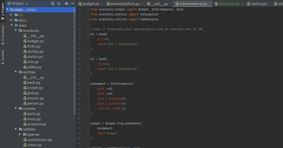
from econtools.budget import Budget, Intertemporal, Good
from econtools.statics import Consumption
from econtools.utility import CobbDouglas
 
# test if intercepts plot appropriately with an interest rate of 10%
m1 = Good(price=1, name='Time 1 Consumption')
 
m2 = Good(price=1, name='Time 2 Consumption')
 
endowment = Intertemporal(
    good_x=m1,
    good_y=m2,
    good_x_quantity=5,
    good_y_quantity=5,
    interest_rate=.10
)
 
budget = Budget.from_endowment(endowment, name='budget')
 
utility = CobbDouglas(.5, 0.5)
 
consumption = Consumption(budget=budget, utility=utility)
 
consumption.show_consumption()

The main thing that sticks out here is that the slope of the budget constraint has changed to reflect the adjustment of income to present value. The x-axis intercept is slightly less than 10 because the present value of income is slightly less than 10, and the y-axis intercept is slightly more than 10 because if a person saved all of their time 1 income, they would receive interest of 5 * .1 = .5, making maximum consumption in period 2 10.5.

Since the person allocates half of the present value of the endowment to time 1 consumption, this means they will spend (5 + 5/1.1) * .5 = 4.77 in period one, saving 5 – 4.77 = .23, which then grows to .23 * (1 + .1) = .25 in period 2, which allows for a time 2 consumption of 5 + .25 = 5.25. This is verified by calling the optimal_bundle() method of the Consumption class:

Python
1
2
consumption.optimal_bundle
Out[7]: (4.7727272727272725, 5.25, 5.005678593539359)

Further Improvements

The Varian chapter on intertemporal choice briefly explores present value calculations for various payment streams, such as bonds and perpetuities. I first made a small attempt at creating a tvm module, but quickly realized that the subject of time value of money is much more complex than what is introduced in Varian, since I know that other texts go further in depth, and hence it may be necessary to split a new repo off from MIES so that it can be distributed separately. This repo is called TmVal, the early stages of which I have uploaded here.

Neither of these are ready for demonstration, but you can click on the links if you are interested in seeing what I have done. The next chapter of Varian covers asset markets, which at first glance seems to just be some examples of economic models, so I’m not sure if it has any features I would like to add to MIES. There is still more work to be done on refactoring the code, so I may do that, or move further into risk aversion, or do some more work on TmVal.
Posted in: Actuarial, MIES / Tagged: economics, insurance, intertemporal choice, MIES

No. 140: MIES – Rate Changes – Slutsky and Hicks Decomposition

28 June, 2020 6:24 PM / Leave a Comment / Gene Dan

This entry is part of a series dedicated to MIES – a miniature insurance economic simulator. The source code for the project is available on GitHub.

Current Status

Last week, I revisited the MIES backend to split what was a single database into multiple databases – one per entity in the simulation. This enhances the level of realism and should make it easier to program transactions between the entities. This week, I’ll revisit consumer behavior by implementing the Slutsky and Hicks decomposition methods for analyzing price changes.

In the context of insurance, consumers frequently experience changes in price, typically during renewals when insurers apply updated rating algorithms against new information known about the insureds. For example, If you’ve made a claim or two during your policy period, and miss a rent payment, causing your credit score to go down, your premium is likely to increase upon renewal. This is because past claims and credit are frequently used as the underlying variables in a rating algorithm.

What happens when consumers face an increase in rates? Oftentimes, they reduce coverage, may try to shop around, or may do nothing at all and simply pay the new price. Today’s post discusses the first phenomenon, whereby an increase in rates causes a reduction in the amount of insurance that a consumer purchases. We can use the Slutsky and Hicks decomposition methods to break down this behavior into two components:

  1. The substitution effect
  2. The income effect

The substitution effect concerns the change in relative prices between two goods. Here, when a consumer faces a premium increase, the price of insurance increases relative to the price of all other goods, altering the rate at which the consumer would be willing to exchange a unit of insurance for a unit of all other goods.

The income effect concerns the change in the price of a good relative to consumer income. When a consumer faces a premium increase without a corresponding increase in income, their income affords them fewer units of insurance.

The content of this post roughly follows the content of chapter 8 in Varian. As usual, I focus on how this applies to my own project and will skip over much of the theoretical derivations that can be found in the text.

Slutsky Identity

The Slutsky identity has the following form:

    \[\frac{\Delta x_1}{\Delta p_1} = \frac{\Delta x_1^s}{\Delta p_1} - \frac{\Delta x_1^m}{\Delta m}x_1\]

Where the x_1 represents the quantity of good 1 (in this case insurance), p_1 represents the price of insurance (that is, the premium) and m represents the consumer’s income. The deltas are used to describe how the quantity of insurance purchased changes with premium, expressed on the left side of the identity. The first term after the equals sign represents the substitution effect, and the second term after the equals sign represents the income effect.

The Slutsky identity can also be expressed in terms of units instead of rates of change (\Delta x_1^m = -\Delta x_1^n):

    \[\Delta x_1 = \Delta x_1^s + \Delta x_1^n\]

While MIES can handle both forms, we’ll focus on the first form for the rest of the chapter.

Substitution Effect

Let’s examine the substitution effect. First, we’ll conduct all the steps manually, and then I’ll show how they are integrated into MIES. If we have some data already stored in a past simulation, we can extract a person from it:

Python
1
2
my_person = Person(1)
my_person.data

1
2
3
4
5
Out[12]:
   person_id age_class profession health_status education_level        income  \
0          1         E          B             F               U  89023.365436  
          wealth  cobb_c  cobb_d  
0  225300.272033     0.1     0.9  

Here, we have a person who makes 89k per year, with Cobb Douglas parameters c = 0.1 and d = 0.9. This means this person will spend 10% of their income on premium. For the sake of making the graphs in this post less cluttered and easier to read, let’s change c = d = .5 so the person spends 50% of their income on insurance:

Python
1
2
3
4
5
6
my_person.utility.c = .5
my_person.utility.d = .5
my_person.get_budget()
my_person.get_consumption()
my_person.get_consumption_figure()
my_person.show_consumption()

From the above figure, we can see that the person consumes about 45k worth of insurance. That’s about 11 units of exposure at a 4k premium per exposure, which is unrealistic in real life, but makes life easy for me because I haven’t bothered to update the margins of my website to accommodate wider figures. We’ll denote this bundle as ‘Old Bundle’ because we’ll compare it to the new consumption bundle after a rate change (note – if you are trying to replicate this in MIES, your figures may look a bit different, in reality I manually adjust the style of the plots so they can fit on my blog).

Now, let’s suppose the person faces a 100% increase in their rate so that their premium is 8k per unit of exposure, and construct a budget to reflect this:

Python
1
2
3
insurance = Good(8000, name='insurance')
all_other = Good(1, name='all other goods')
new_budget = Budget(insurance, all_other, income=my_person.income, name='new_budget')

Plotting this new budget, we see that the line tilts inward, since the person can only afford half as much insurance as before:

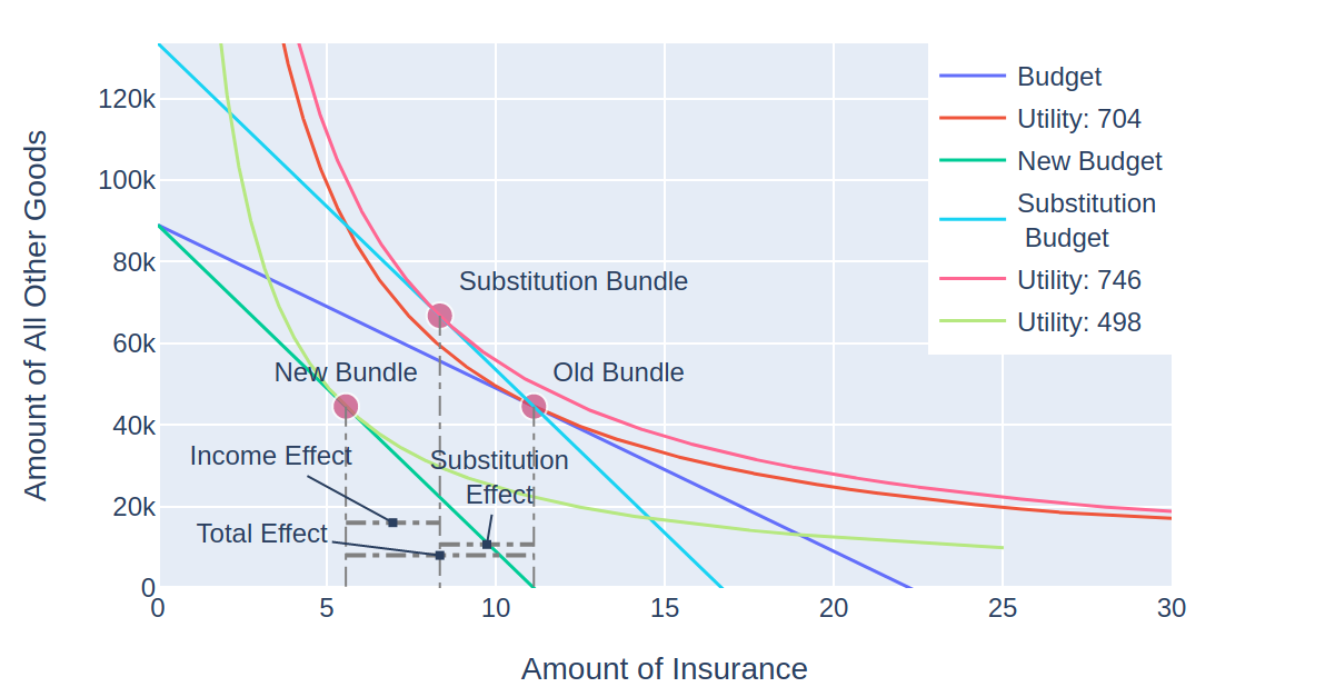
The first stage in Slutsky decomposition involves calculating the substitution effect. This is done by tilting the budget line to the slope of the new prices, but with income adjusted so that the person can still afford their old bundle. We then determine the new optimal bundle at this budget (denoted ‘substitution budget’) and call it the substitution bundle:

    \[\Delta m = x_1 \Delta p_1\]

1
2
3
sub_income = my_person.income + my_person.optimal_bundle[0] * 4000
substitution_budget = Budget(insurance, all_other, income=sub_income, name='Substitution<br /> Budget')
...more plotting code...

You can see that if the person were given enough money to purchase the same amount of insurance even after the rate increase, they would still reduce their consumption from 11.1 to 8.3 units of insurance. 8.3 – 11.1 = -2.8 is the substitution effect.

Income Effect

Now, to calculate the income effect, we then shift the substitution budget to the position of the new budget:

The person purchases 5.5 units of insurance at the new budget, so the income effect is 5.5 – 8.3 = -2.8 for the substitution effect. The total effect is -2.8 -2.8 = -5.6 units of insurance, the sum of the substitution and income effect. This is the same as the new consumption minus the old consumption 5.5 – 11.1 = -5.6

MIES Integration

The Slutsky decomposition process has been integrated into MIES as a class in econtools/slutsky.py:

Python
1
2
3
4
5
6
7
8
9
10
11
12
13
14
15
16
17
18
19
20
21
22
23
24
25
26
27
28
29
30
31
32
33
34
35
36
37
38
39
40
41
42
43
44
45
46
47
48
49
50
51
52
53
54
55
56
57
58
59
60
61
62
63
64
65
66
67
68
69
70
71
72
73
74
75
76
77
78
79
80
81
82
83
84
85
86
87
88
89
90
91
92
93
94
95
96
97
98
99
100
101
102
103
104
105
106
107
108
109
110
111
112
113
114
115
116
117
118
119
120
121
122
123
124
125
126
127
128
129
130
131
132
133
134
135
136
137
138
139
140
141
142
143
144
145
146
147
148
149
150
151
152
153
154
155
156
157
158
159
160
161
162
163
164
165
166
167
168
169
170
171
172
173
174
175
176
177
178
179
180
181
182
183
184
185
186
187
188
189
190
191
192
193
194
195
196
197
198
199
200
201
202
203
204
205
206
207
208
209
210
211
212
213
214
215
216
217
218
219
220
221
222
223
224
225
226
227
228
229
230
231
232
233
234
235
236
237
238
239
240
241
242
243
244
245
246
247
248
249
250
251
252
253
254
255
256
257
258
259
260
261
262
263
264
265
266
267
268
269
270
271
272
273
274
275
276
277
278
279
280
281
282
283
284
285
286
287
288
289
290
291
292
293
294
295
296
297
298
299
300
301
302
303
304
305
306
307
308
309
310
311
312
313
314
315
316
317
318
319
320
321
322
323
324
325
326
import plotly.graph_objects as go
 
from plotly.offline import plot
from econtools.budget import Budget
from econtools.utility import CobbDouglas
 
 
class Slutsky:
    """
    Implementation of the Slutsky equation, accepts two budgets, a utility function, and calculates
    the income and substitution effects
    """
    def __init__(
            self,
            old_budget: Budget,
            new_budget: Budget,
            utility_function: CobbDouglas  # need to replace with utility superclass
    ):
        self.old_budget = old_budget
        self.old_budget.name = 'Old Budget'
        self.new_budget = new_budget
        self.new_budget.name = 'New Budget'
        self.utility = utility_function
 
        self.old_bundle = self.utility.optimal_bundle(
            self.old_budget.good_x.price,
            self.old_budget.good_y.price,
            self.old_budget.income
        )
 
        self.delta_p = self.new_budget.good_x.price - self.old_budget.good_x.price
        self.pivoted_budget = self.calculate_pivoted_budget()
        self.substitution_bundle = self.calculate_substitution_bundle()
        self.substitution_effect = self.calculate_substitution_effect()
        self.new_bundle = self.calculate_new_bundle()
        self.income_effect = self.calculate_income_effect()
        self.total_effect = self.substitution_effect + self.income_effect
        self.substitution_rate = self.calculate_substitution_rate()
        self.income_rate = self.calculate_income_rate()
        self.slutsky_rate = self.substitution_rate - self.income_rate
        self.plot = self.get_slutsky_plot()
 
    def calculate_pivoted_budget(self):
        """
        Pivot the budget line at the new price so the consumer can still afford their old bundle
        """
        delta_m = self.old_bundle[0] * self.delta_p
        pivoted_income = self.old_budget.income + delta_m
        pivoted_budget = Budget(
            self.new_budget.good_x,
            self.old_budget.good_y,
            pivoted_income,
            'Pivoted Budget'
        )
        return pivoted_budget
 
    def calculate_substitution_bundle(self):
        """
        Return the bundle consumed after pivoting the budget line
        """
        substitution_bundle = self.utility.optimal_bundle(
            self.pivoted_budget.good_x.price,
            self.pivoted_budget.good_y.price,
            self.pivoted_budget.income
        )
        return substitution_bundle
 
    def calculate_substitution_effect(self):
        substitution_effect = self.substitution_bundle[0] - self.old_bundle[0]
        return substitution_effect
 
    def calculate_new_bundle(self):
        """
        Shift the budget line outward
        """
        new_bundle = self.utility.optimal_bundle(
            self.new_budget.good_x.price,
            self.new_budget.good_y.price,
            self.new_budget.income
        )
        return new_bundle
 
    def calculate_income_effect(self):
        income_effect = self.new_bundle[0] - self.substitution_bundle[0]
        return income_effect
 
    def calculate_substitution_rate(self):
        delta_s = self.calculate_substitution_effect()
        delta_p = self.new_budget.good_x.price - self.old_budget.good_x.price
        substitution_rate = delta_s / delta_p
        return substitution_rate
 
    def calculate_income_rate(self):
        delta_p = self.new_budget.good_x.price - self.old_budget.good_x.price
        delta_m = self.old_bundle[0] * delta_p
        delta_x1m = -self.calculate_income_effect()
        income_rate = delta_x1m / delta_m * self.old_bundle[0]
        return income_rate
 
    def get_slutsky_plot(self):
        max_x_int = max(
            self.old_budget.income / self.old_budget.good_x.price,
            self.pivoted_budget.income / self.pivoted_budget.good_x.price,
            self.new_budget.income / self.new_budget.good_x.price
        ) * 1.2
 
        max_y_int = max(
            self.old_budget.income,
            self.pivoted_budget.income,
            self.new_budget.income,
        ) * 1.2
 
        # interval boundaries
        effect_boundaries = [
            self.new_bundle[0],
            self.substitution_bundle[0],
            self.old_bundle[0]
        ]
        effect_boundaries.sort()
 
        fig = go.Figure()
 
        # budget lines
        fig.add_trace(self.old_budget.get_line())
        fig.add_trace(self.pivoted_budget.get_line())
        fig.add_trace(self.new_budget.get_line())
 
        # utility curves
        fig.add_trace(
            self.utility.trace(
                k=self.old_bundle[2],
                m=max_x_int,
                name='Old Utility'
            )
        )
        fig.add_trace(
            self.utility.trace(
                k=self.substitution_bundle[2],
                m=max_x_int,
                name='Pivoted Utility'
            )
        )
        fig.add_trace(
            self.utility.trace(
                k=self.new_bundle[2],
                m=max_x_int,
                name='New Utility'
            )
        )
        # consumption bundles
 
        fig.add_trace(
            go.Scatter(
                x=[self.old_bundle[0]],
                y=[self.old_bundle[1]],
                mode='markers+text',
                text=['Old Bundle'],
                textposition='top center',
                marker=dict(
                    size=[15],
                    color=[1]
                ),
                showlegend=False
            )
        )
 
        fig.add_trace(
            go.Scatter(
                x=[self.substitution_bundle[0]],
                y=[self.substitution_bundle[1]],
                mode='markers+text',
                text=['Pivoted Bundle'],
                textposition='top center',
                marker=dict(
                    size=[15],
                    color=[2]
                ),
                showlegend=False
            )
        )
 
        fig.add_trace(
            go.Scatter(
                x=[self.new_bundle[0]],
                y=[self.new_bundle[1]],
                mode='markers+text',
                text=['New Bundle'],
                textposition='top center',
                marker=dict(
                    size=[15],
                    color=[3]
                ),
                showlegend=False
            )
        )
        # Substitution and income effect interval lines
        fig.add_shape(
            type='line',
            x0=self.substitution_bundle[0],
            y0=self.substitution_bundle[1],
            x1=self.substitution_bundle[0],
            y1=0,
            line=dict(
                color="grey",
                dash="dashdot",
                width=1
            )
        )
 
        fig.add_shape(
            type='line',
            x0=self.new_bundle[0],
            y0=self.new_bundle[1],
            x1=self.new_bundle[0],
            y1=0,
            line=dict(
                color="grey",
                dash="dashdot",
                width=1
            )
        )
 
        fig.add_shape(
            type='line',
            x0=self.old_bundle[0],
            y0=self.old_bundle[1],
            x1=self.old_bundle[0],
            y1=0,
            line=dict(
                color="grey",
                dash="dashdot",
                width=1
            )
        )
        fig.add_shape(
            type='line',
            xref='x',
            yref='y',
            x0=effect_boundaries[0],
            y0=max_y_int / 10,
            x1=effect_boundaries[1],
            y1=max_y_int / 10,
            line=dict(
                color='grey',
                dash='dashdot'
            )
        )
        fig.add_shape(
            type='line',
            xref='x',
            yref='y',
            x0=effect_boundaries[1],
            y0=max_y_int / 15,
            x1=effect_boundaries[2],
            y1=max_y_int / 15,
            line=dict(
                color='grey',
                dash='dashdot'
            )
        )
        fig.add_shape(
            type='line',
            xref='x',
            yref='y',
            x0=effect_boundaries[0],
            y0=max_y_int / 20,
            x1=effect_boundaries[2],
            y1=max_y_int / 20,
            line=dict(
                color='grey',
                dash='dashdot'
            )
        )
 
        fig.add_annotation(
            x=(self.substitution_bundle[0] + self.old_bundle[0]) / 2,
            y=max_y_int / 10,
            text='Substitution<br />Effect',
            xref='x',
            yref='y',
            showarrow=True,
            arrowhead=7,
            ax=5,
            ay=-40,
        )
 
        fig.add_annotation(
            x=(self.new_bundle[0] + self.substitution_bundle[0]) / 2,
            y=max_y_int / 15,
            text='Income Effect',
            xref='x',
            yref='y',
            showarrow=True,
            arrowhead=7,
            ax=50,
            ay=-20
        )
 
        fig.add_annotation(
            x=(effect_boundaries[2] + effect_boundaries[0]) / 2,
            y=max_y_int / 20,
            text='Total Effect',
            xref='x',
            yref='y',
            showarrow=True,
            arrowhead=7,
            ax=100,
            ay=20
        )
 
        fig['layout'].update({
            'title': 'Slutsky Decomposition',
            'title_x': 0.5,
            'xaxis': {
                'title': 'Amount of Insurance',
                'range': [0, max_x_int]
            },
            'yaxis': {
                'title': 'Amount of All Other Goods',
                'range': [0, max_y_int]
            }
        })
        return fig
 
    def show_plot(self):
        plot(self.plot)

This has been added to the Person class, so we can use its methods to get the substitution and income effects. This conveniently packages all the manual steps we took above together:

Python
1
2
3
my_person.calculate_slutsky(new_budget)
my_person.slutsky.income_effect
my_person.slutsky.substitution_effect

Which returns -2.8 for each effect, the same as above.

Hicks Decomposition

A similar decomposition method is called Hicks decomposition. Instead of pivoting the budget constraint so that the person can afford the same bundle as before, the budget constraint is shifted so that they have the same utility as before. Using algebra, we can solve this by fixing utility:

    \[m^\prime = \frac{\bar{u}}{\left(\frac{c}{c +d}\frac{1}{p_1^\prime}\right)^c\left(\frac{d}{c+d}\frac{1}{p_2}\right)^d}\]

where m^\prime is the adjusted income, and p_1^\prime is the new premium, and \bar{u} is the utility fixed at the original level.

You’ll notice there’s a subtle difference, the new bundle is the same as in the Slutsky case, but the substitution bundle in this case is on the original utility curve. This gives different answers for the substitution and income effects, which are -3.3 and -2.3, which add up to a total effect of -5.6, as before.

The code for the Hicks class is much the same as that for the Slutsky class, so I won’t post most of it here, the relevant change is in calculating the substitution budget:

Python
1
2
3
4
5
6
7
8
9
10
11
12
13
14
15
16
17
18
19
20
21
22
23
class Hicks:
...
 
    def calculate_pivoted_budget(self):
        """
        Pivot the budget line at the new price so the consumer still as the same utility
        """
        old_utility = self.old_bundle[2]
        c = self.utility.c
        d = self.utility.d
        p1_p = self.new_budget.good_x.price
        p2 = self.old_budget.good_y.price
        x1_no_m = (((c / (c + d)) * (1 / p1_p)) ** c)
        x2_no_m = (((d / (c + d)) * (1 / p2)) ** d)
        pivoted_income = old_utility / (x1_no_m * x2_no_m)
        pivoted_budget = Budget(
            self.new_budget.good_x,
            self.old_budget.good_y,
            pivoted_income,
            'Pivoted Budget'
        )
        return pivoted_budget
        ...

Further Improvements

Since Hicks substitution is mostly similar to Slutsky in terms of code, it makes sense for the Hicks class to inherit from the Slutsky class or for both of them to inherit from a superclass.

I’m currently working on implementing wealth into MIES, since as of today, none of the transactions actually impact wealth.

Posted in: Actuarial, Mathematics, MIES / Tagged: actuarial, insurance, MIES, simulator

No. 132: Exploring Serverless Architectures for MIES

21 April, 2019 9:44 PM / Leave a Comment / Gene Dan

A few months ago, I introduced MIES, an insurance simulation engine. Although I wanted to work on this for the last few years, I had been sidetracked with exams, and more recently, a research project for the Society of Actuaries (SOA) that involved co-authoring a predictive modeling paper with other actuaries and data scientists at Milliman. That effort took an entire year from the initial proposal to its final publication, of which the copy-edit stage is still ongoing. Once it has been published, I’ll provide another update on my thoughts over the whole process.

Meanwhile, I’ve had some time to get back to MIES. As far as technology goes, a lot has changed over the years, including the introduction of serverless computing – implemented in AWS Lambda in 2014. In short, serverless computing is a cloud service that allows you to execute code without having to provision or configure servers or virtual machines. Furthermore, you only need to pay for what you execute, and there is no need to terminate clusters or machines in order to save on costs. Ideally, this should be more cost (and time) effective than other development options that involve allocating hardware.

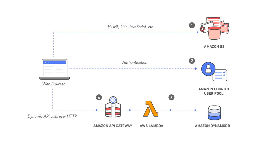
Since MIES is cloud-based, I thought going serverless would be worth a try, and was further motivated to do so upon the recommendation of a friend. The following image comes from one of the AWS tutorials on serverless web apps. What I have envisioned is similar, with the exception of using Postgres instead of DynamoDB.

Following the tutorial was easy enough, and took about two hours to complete. My overall assessment is that although I was able to get the web app up and running quickly, many of the pieces of the tutorial, such as the files used to construct the web page, and the configuration options for the various AWS services involved (S3, Cognito, DynamoDB, Lambda, API Gateway) were preset without explanation, which made it hard to really understand how the architecture worked, or what all the configuration options did, or why they were necessary. Furthermore, I think a developer would need to have more experience in the component AWS services to be able to build their own application from scratch. Nevertheless, I was impressed enough to want to continue experimenting with serverless architectures for MIES, so I purchased two books to get better at both AWS itself and AWS Lambda:

  1. Amazon Web Services in Action
  2. AWS Lambda in Action

One downside to this approach is that while informative, these types of books tend to go out of date quickly – especially in the case of cloud technologies. For example, I have read some books on Spark that became obsolete less than a year after publication. On the other hand, books offer a structured approach to learning that can be more organized and approachable than reading the online documentation or going to Stack Overflow for every problem that I encounter. This is however, cutting edge technology, and no one approach will cover everything I’ll need to learn. I’ll have to take information wherever I can get it, and active involvement in the community is a must when trying to learn these things.

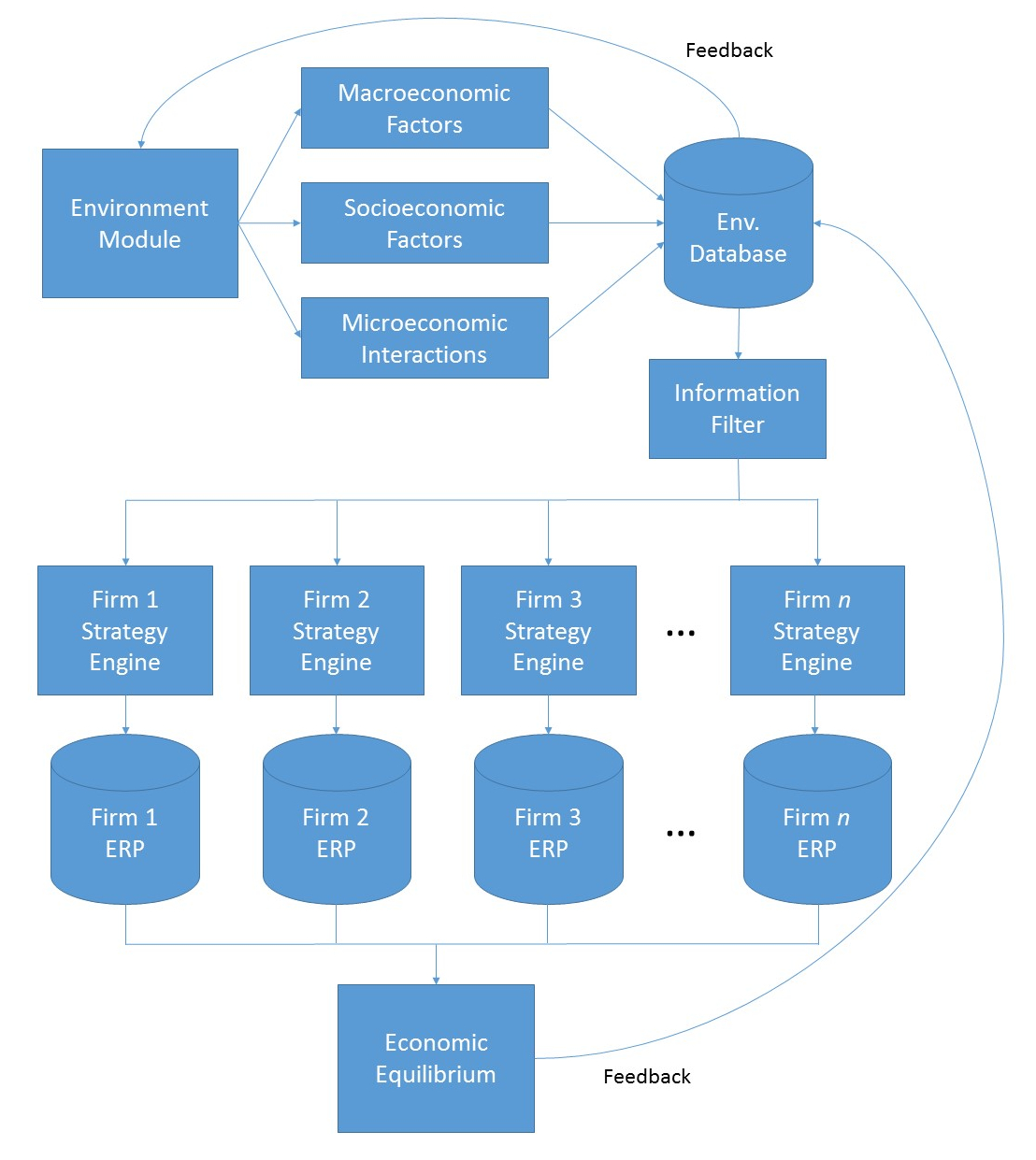
Going back to the original MIES diagram, we can see that serverless computing is ideal:

I ought to be able to program the modules in AWS Lambda and store the data in Postgres instances. Having multiple firms will complicate things, as will focusing on the final display of information, along with the user interface. For now, I’ll focus on generating losses for one firm, and then reaching an equilibrium with 2 firms. I already have a schema mocked up in Postgres, and will work on connecting to it with Python over the course of the week.

Posted in: MIES / Tagged: MIES

No. 130: Introducing MIES – A Miniature Insurance Economic Simulator

26 November, 2018 12:31 AM / Leave a Comment / Gene Dan

MIES, standing for Miniature Insurance Economic Simulator, is a side project of mine that was originally conceived in 2013. The goal of MIES is to create a realistic, but simplified representation of an insurance company ERP, populate it with simulated data, and from there use it to test economic and actuarial theories found in academic literature. From this template, multiple firms can then be created, which can then be used to test inter-firm competition, the effects of which will be manifested via the simulated population of insureds.
Inspiration for the project came from the early days of my career, when I was first learning how to program computers. While I found ample general-purpose material online for popular languages such as Python, R, and SQL, little existed as far as insurance-specific applications. Likewise, from an insurance perspective, plenty of papers were available from the CAS, but they were mostly theoretical in nature and lacked the practical aspects of using numerical programming to conduct actuarial work – i.e., using SQL to pull from databases, what a typical insurance data warehouse looks like, how to build a pricing model with R, etc.

I had hoped to bridge that gap by creating a mock-up of an insurance data warehouse that could be used to practice SQL queries against, thus bridging the gap between theory and practice, and creating a resource that other actuaries and students could use to further their own education. I then realized that not only would I be able to simulate a single company’s operations, but I’d also be able to simulate firm interactions by cloning the database template and deploying competing firm strategies against each other. And furthermore, should I succeed in creating a robust simulation engine, I would be able to incorporate and test open source actuarial libraries written by others.

I would have liked to introduce this project later, but I figured if I were to reveal pieces of the project (like I did with the last post) without an overarching framework, readers wouldn’t really get the point of what I was trying to achieve. Back in 2013, the project stalled due to exams, and my lack of technical knowledge and insurance experience. Now that I’ve worked for a bit and finished my exams, I can continue work on this more regularly. Below, I present a high-level schematic of the MIES engine:

The image above displays two of the three layers of the engine – an environment layer that is used to simulate the world in which firms and the individuals they hope to insure interact, and a firm layer that stores each firm’s ERP and corporate strategy.

  • Environment Layer
  • The environment layer simulates the population of potential insureds who are subject to everyday perils that insurance companies hope to insure. The environment module will be a program (or collection of programs) that provides the macroeconomic (GDP, unemployment, inflation), microeconomic (individual wealth, utility curves, births and deaths), sociodemographic (race, religion, household income, commute time), and other environmental parameters such as weather, to represent everyday people and the challenges they face. The simulated data are stored in a database (or a portion of a very large database) called the environmental database.

    A module called the information filter then reads the environmental data and filters out information that can’t be seen by individual firms. Firms try to get as much data as they can about their potential customers, but they won’t be able to know everything about them. Therefore, firms act on incomplete information, and the information filter is designed to remove information that companies can’t access.

  • Firm Layer
  • The firm layer is a collection of firm strategies – each of which is a program that represents the firm’s corporate strategy (pricing, reserving, marketing, claims, human resources, etc.), along with a set of firm ERPs which store the information resulting from each firm’s operations (premiums, claims, financial statements, employees).

The environment layer then simulates policies written and claims incurred, which are then stored in their respective firm’s ERPs. The result of all this is a set of economic equilibria – that is, insurance market prices, adequacy, availability, etc. Information generated from both the environment and firm layers are then fed back into the environment module as a form of feedback that influences the next iteration’s simulation.

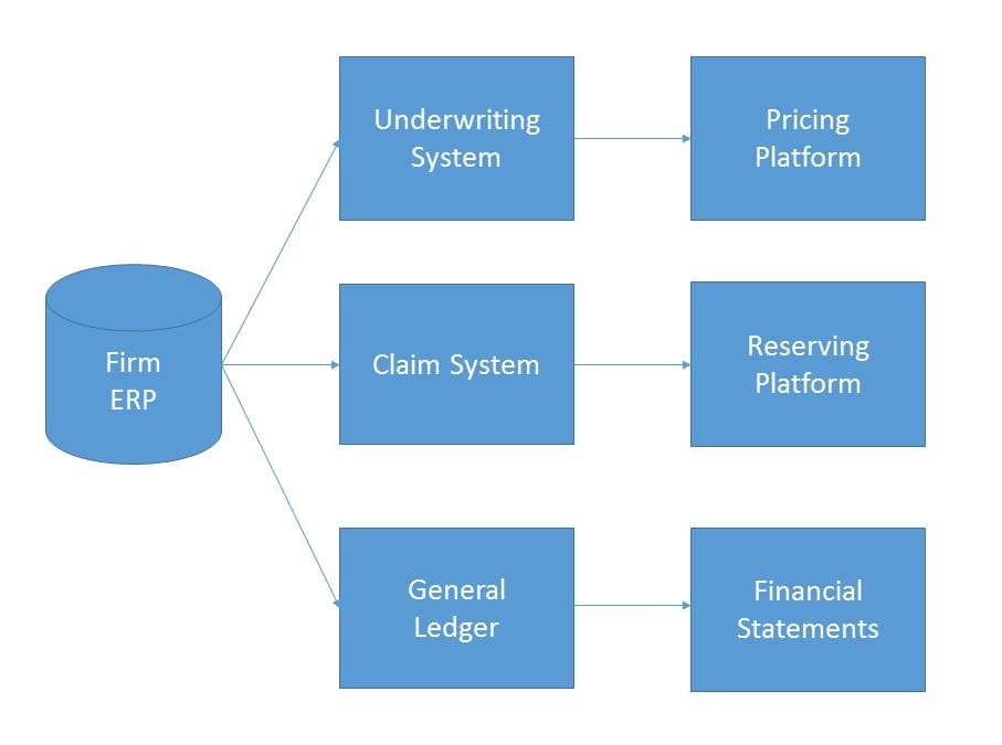
The image below represents a simple breakdown of an individual firm ERP:

Here, we have the third layer of MIES – the user interface layer.

  • Underwriting System
  • An underwriting system is a platform that an insurer uses to write policies. I’ll try my best to use an available open-source engine for this (possibly openunderwriter). The frontend will be visible if a human actor is involved, otherwise, it will be driven behind the scenes programmatically.

  • Claims System
  • A claims system is a platform that an insurer uses to manage and settle insurance claims. On top of the claims system is the actuarial reserving interface (triangles).

  • General Ledger
  • The general ledger stores accounting information that is used to produce financial statements. Current candidates for this system include ledger-cli and LedgerSMB.

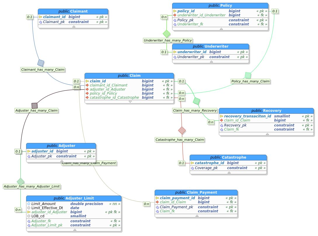
Below, is a rudimentary claims database schema, containing primary-foreign key relationships, but no other attributes (to be added later):

I’m using PostgreSQL for the database system, and MIES itself will be hosted on my AWS cloud account as a web-based application. I’m currently exploring Apache and serverless options as a host. The MIES engine itself was originally being scripted in Scala (I was really into Spark at the time) but will now be done in Python to reach a wider audience (I may revisit Scala if the data becomes big – hopefully I’ll be able to get some kind of funding for hosting fees if that happens).

With this ecosystem, I aim to reconcile micro- and macroeconomic theory, and study the effects of firm competition, oligopoly, and bankruptcy on the well-being of insureds. The engine will serve as the basis for other actuarial libraries and will incorporate pricing, reserving, and ERP systems that could eventually become standalone open-source applications for the insurance industry. Stay tuned for updates, and check the github repo regularly to see the project progress.

Posted in: Uncategorized / Tagged: actuarial science, insurance, MIES

Archives

  • September 2023
  • February 2023
  • January 2023
  • October 2022
  • March 2022
  • February 2022
  • December 2021
  • July 2020
  • June 2020
  • May 2020
  • May 2019
  • April 2019
  • November 2018
  • September 2018
  • August 2018
  • December 2017
  • July 2017
  • March 2017
  • November 2016
  • December 2014
  • November 2014
  • October 2014
  • August 2014
  • July 2014
  • June 2014
  • February 2014
  • December 2013
  • October 2013
  • August 2013
  • July 2013
  • June 2013
  • March 2013
  • January 2013
  • November 2012
  • October 2012
  • September 2012
  • August 2012
  • July 2012
  • June 2012
  • May 2012
  • April 2012
  • March 2012
  • February 2012
  • January 2012
  • December 2011
  • September 2011
  • August 2011
  • July 2011
  • June 2011
  • January 2011
  • December 2010
  • October 2010
  • September 2010
  • August 2010
  • June 2010
  • May 2010
  • April 2010
  • March 2010
  • September 2009
  • August 2009
  • May 2009
  • December 2008

Categories

  • Actuarial
  • Cycling
  • Logs
  • Mathematics
  • MIES
  • Music
  • Uncategorized

Links

Cyclingnews
Jason Lee
Knitted Together
Megan Turley
Shama Cycles
Shama Cycles Blog
South Central Collegiate Cycling Conference
Texas Bicycle Racing Association
Texbiker.net
Tiffany Chan
USA Cycling
VeloNews

Texas Cycling

Cameron Lindsay
Jacob Dodson
Ken Day
Texas Cycling
Texas Cycling Blog
Whitney Schultz
© Copyright 2025 - Gene Dan's Blog
Infinity Theme by DesignCoral / WordPress