• Home
  • Readings
  • Github
  • MIES
  • TmVal
  • About
Gene Dan's Blog

Author Archives: Gene Dan

No. 147: The Chain Ladder Method with FASLR

27 March, 2022 4:25 PM / 1 Comment / Gene Dan

Today marks an exciting milestone – FASLR (Free Actuarial System for Loss Reserving) – has now implemented its first reserving technique, the chain ladder method. This makes it a good time to update the version number for the project, so I’ve bumped it from its inception v0.0.0 to v0.0.1. Feel free to check out the source code on the CAS GitHub.

New features added:

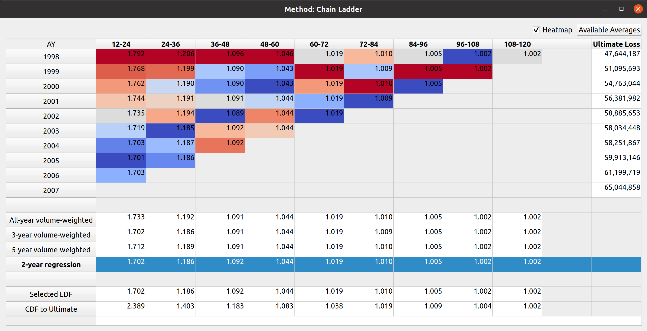
  • Ultimate Loss Column calculated via the chain ladder technique
  • Rows for selected LDFs and CDFs
  • The ability to select LDFs by double-clicking averages
  • Dialog box for creating and storing custom link ratio average types
  • Link ratio heatmap

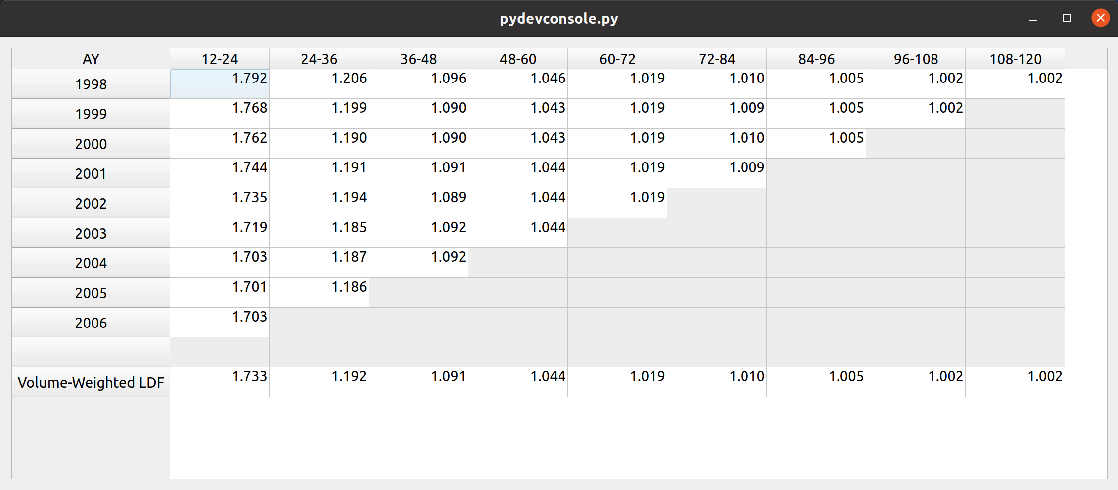
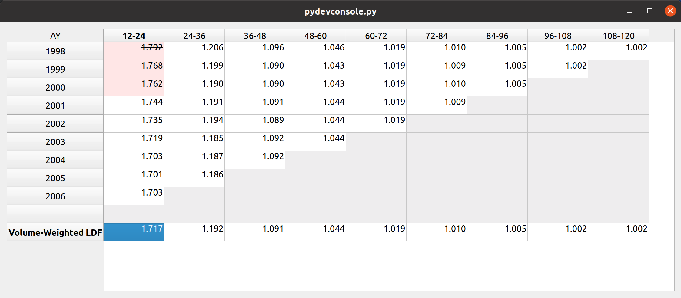
These features have been added to the development factor view of FASLR. The images below show a comparison to how it looked last month (first image) vs. how it looks now, with the new features highlighted in red boxes (second image):

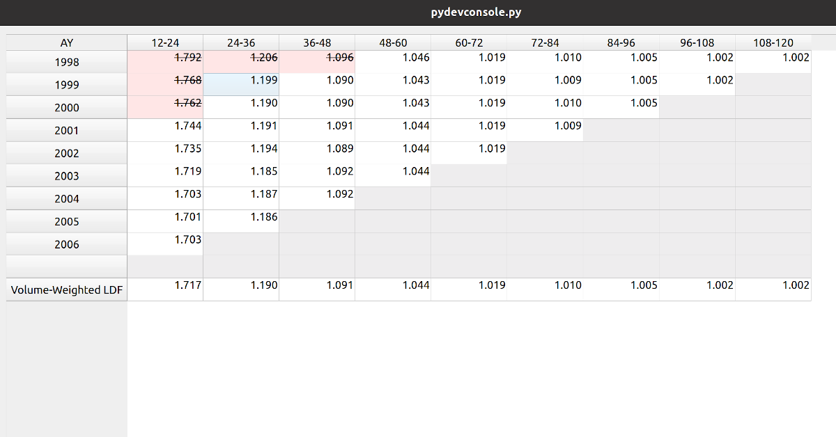
The FASLR development view, last month.

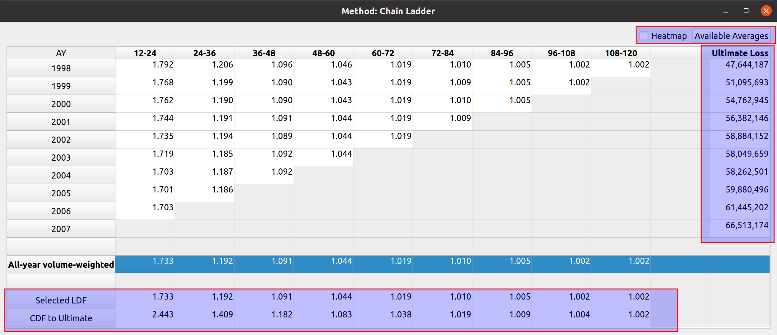
The FASLR development view, newest version.

Project Status

When examining the views of the repo, I’ve seen a lot of people taking a look at the releases section, the setup.py file, and the documentation. This leads me to believe that some people either think this is an installable program or are checking to see if it is. Right now, the project exists as a collection of Python source code files, so it’s not there yet. I do have plans to eventually release installable binaries where you can just double click a file and have it installed on your operating system. But first, I would have to learn how to do that and I have yet to decide on which tool I want to use to make that happen (GNU Make, Bazel, fbs, pyinstaller, etc.). This will be a new skill for me to acquire so it will take some time.

If you do want to run FASLR, you can execute the file main.py in the shell. This will give you access to the main GUI window and project pane. Currently, I’m focused on setting up views for the various reserving methodologies, once I’ve either exhausted those available in the chainladder package, or reached a point where it would be nice to integrate them into the main window, I will begin to focus more on the reserving project methodology – i.e., making it possible to start from data importation and end with a reserving estimate.

Versioning Methodology

The versioning system consists of a three-part format: v#.#.#. The rightmost digit represents unstable versions. Excluding v0.0.0, if your installation happens to have a rightmost digit other than 0, you can assume that you are using the software for the purpose of testing out the latest features and not relying on stability. The middle digit represents stable releases, meaning that the features have been tested to the best of the ability of the developer(s) and provide a reasonable level of reliability. So something like v0.1.0 would represent the first stable version and v0.1.1 would represent the most recent unstable version released after v0.1.0. The next stable version after v0.1.0 will be v0.2.0.

The leftmost digit represents major cultural milestones in the project. Right now it seems to be in vogue to reserve version 1.whatever for a special occasion, to mark the point where the software has become the de-facto open-source standard for performing work in the field. I will adopt this convention for this project, but while I have no plans to ever reach this point, as FASLR is mostly a learning exercise for me, it would be a nice point to reach if it ever gains traction.

Ultimate Losses

Since there are numerous sources on actuarial reserving methods which can do a much better job of explaining how they work than I can, I won’t spend much detail here on them and you can always refer back to CAS Exam 5 papers if you are not familiar with them. These next few sections will start with a blank factor view, and I will gradually demonstrate how link ratio averages can be used, in combination with the chain ladder technique to project ultimate loss.

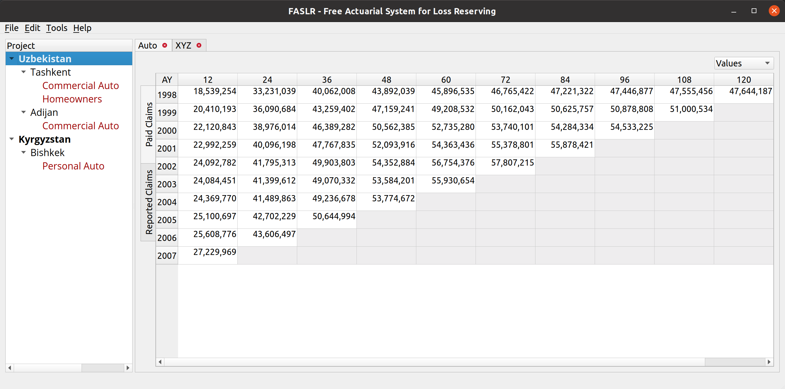
One purpose of actuarial reserving is to estimate the liabilities per unit of time (such as accident year) and we call this estimate the ultimate loss. Therefore, one of my goals for this month was to add a column for ultimate loss. Below shows the (mostly) blank factor view with the link ratio triangle and ultimate loss column to the right. The LDFs have not been selected, and the chainladder package defaults non-selection to 1.000:

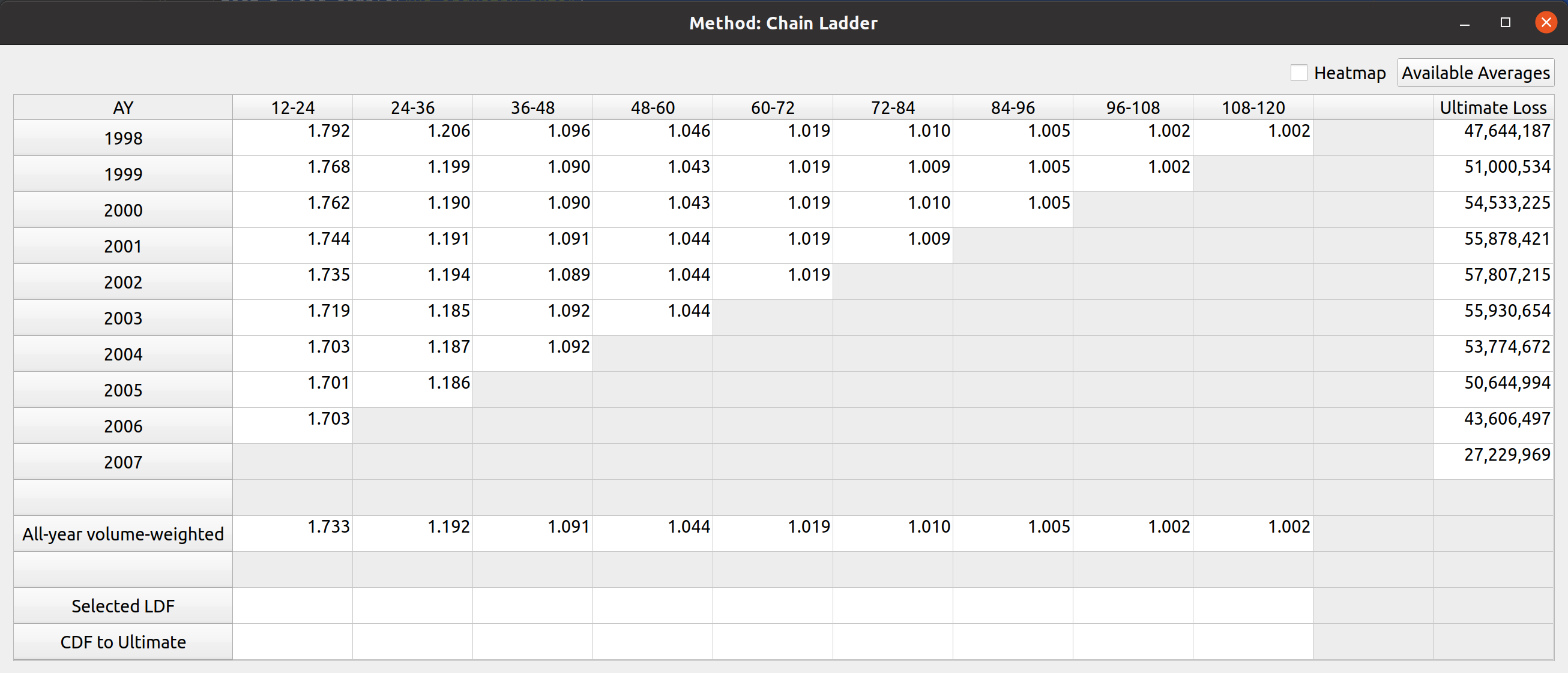
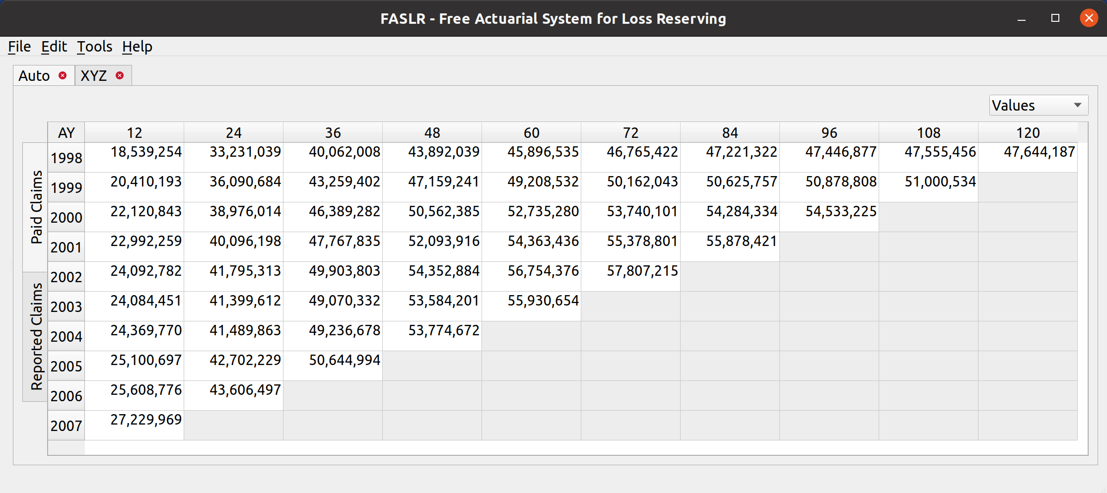
You can confirm that the starting LDFs are 1.000 by looking at the source triangle – the ultimate loss values are the same as the latest diagonal:

LDF Selection

Below the triangle, you will find a section that has various link ratio averages that you can select by double-clicking on them. The image in the previous section only had one option, the all-year volume-weighted average, but you can add more by selecting the “Available Averages” button in the upper-right hand corner. Doing so will open up a dialog box with averages that you can add to the factor view:

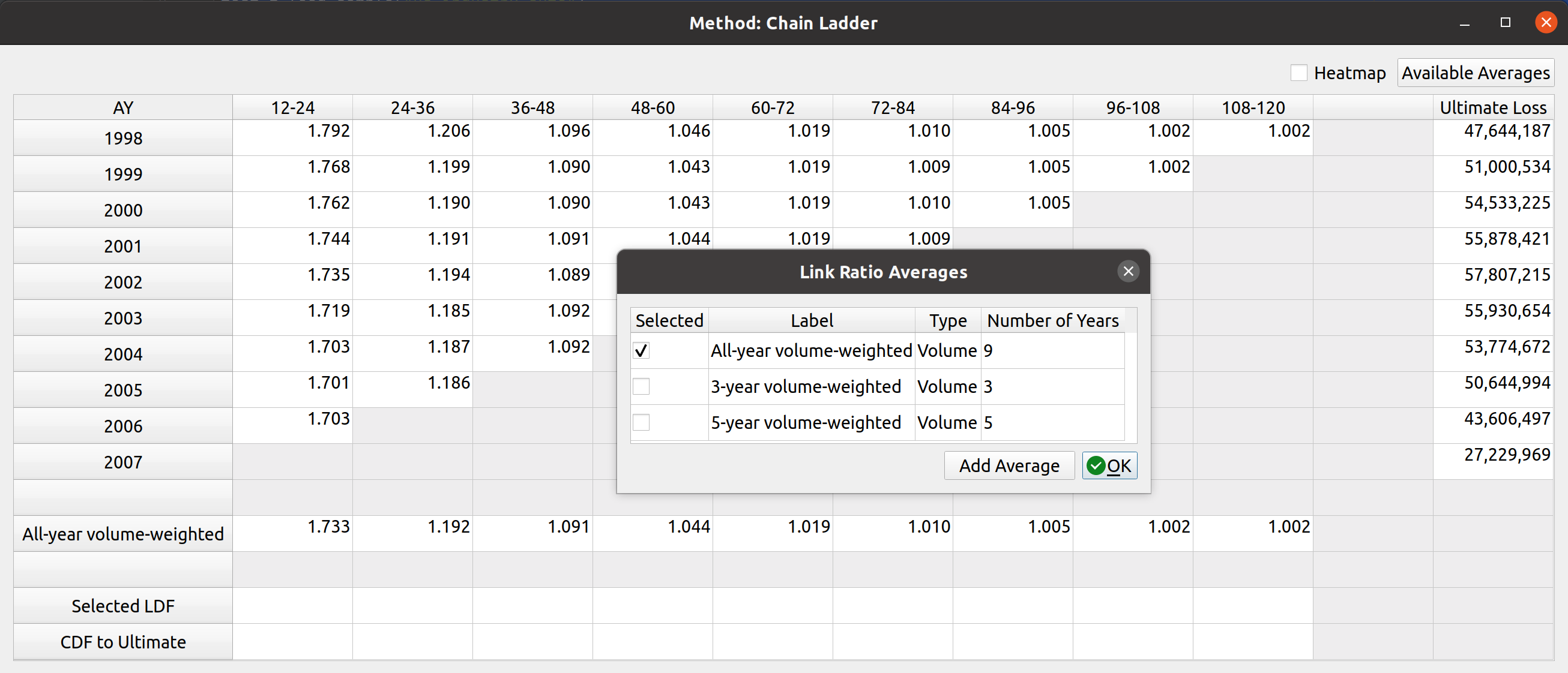
The starting averages are All, 5-, and 3- year volume-weighted averages. You can add these by clicking the checkboxes in the table. Alternatively, you can add a custom type if you want to use a different kind of average like straight or regression. You can do this by clicking the “Add Average” button and then selecting the options for the new average. Right now, only these three are supported by chainladder, but I have proposed that we add others like medial and geometric to the list:

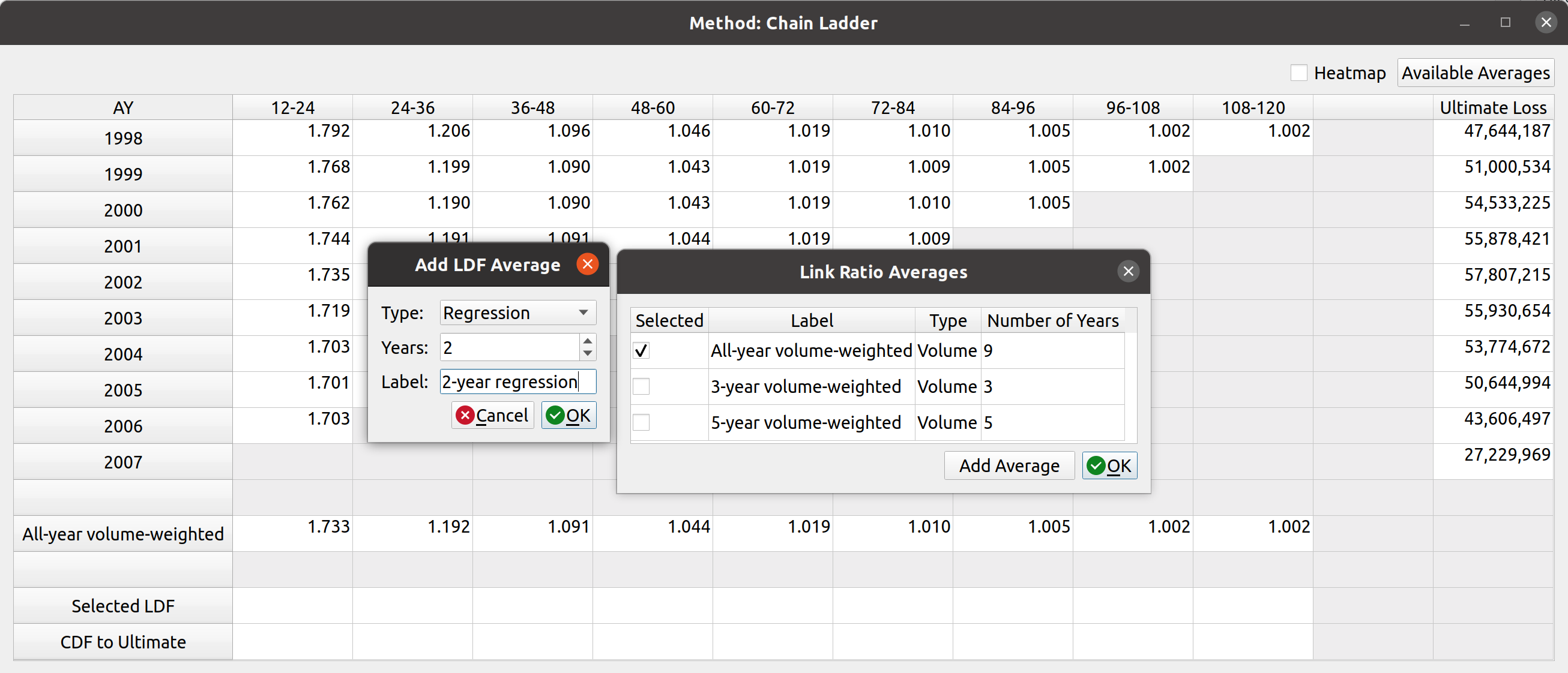
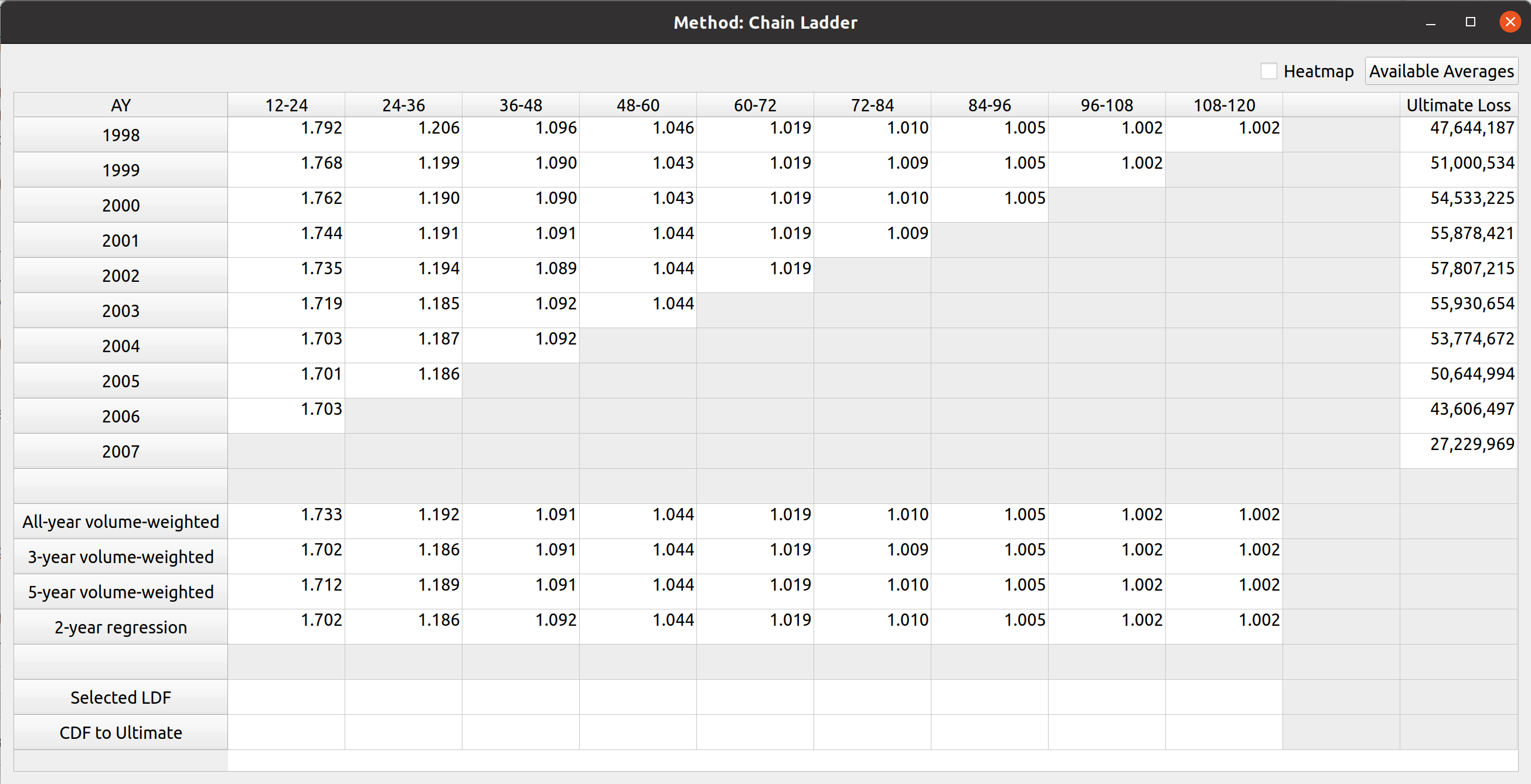
In this example I have added a 2-year regression and selected all 4 average types in the table. This expands the number of rows in the LDF section of the factor view:

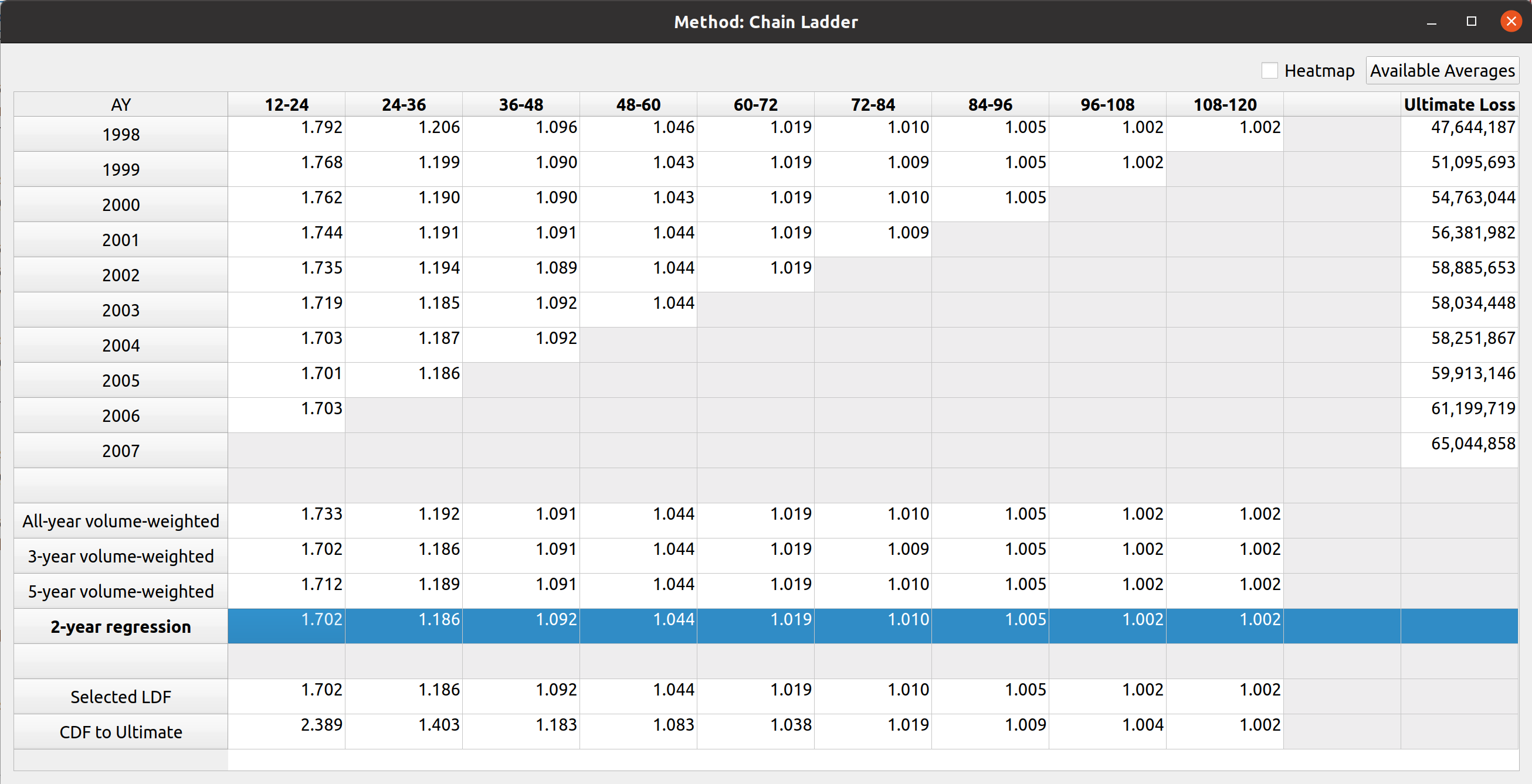
Next, you can select the LDFs by double-clicking on the LDF section. Double-clicking an entire row will select that whole row, and the CDFs are automatically calculated. The image below shows that I have selected the 2-year regression, and the ultimate loss values are automatically updated:

Alternatively, you can enter in your own custom values by typing or copy-pasting into the cells directly. And you can delete the selections by pressing the delete key over the cells or by double-clicking the row header of the selected LDF row. You can also remove LDF average types by clicking on the “available averages” button and unchecking the ones you want to remove.

Heatmap

This last feature is something that comes from the chainladder package. It was quite challenging to implement even though on the surface, all you have to do is tick the checkbox. This helps you identify outlier link ratios that you may want to exclude in your analysis:

There are some performance enhancements to be made on this feature, I’ll write up another post once that’s done. Below, you’ll see a gif of all of what I described above in action:

Posted in: Actuarial

No. 146: Development Factors with FASLR

21 February, 2022 5:42 PM / Leave a Comment / Gene Dan

A few things have happened since this last time I’ve posted about a technical subject – I have gotten into contact with Brian Fannin over at the CAS and now have two projects hosted on their GitHub page – PCDM, which I wrote about a couple years ago, and FASLR, a new project I started last year, which I’ll be talking about today.

FASLR (pronounced fæzlɹ̩), is a GUI wrapper built using the PyQt framework to accommodate open-source actuarial reserving engines, such as the chainladder packages written in Python and R.

OK. The buzzword-free version of that sentence is that FASLR is open-source software that is intended to help actuaries do reserving with buttons, windows, and mouse clicks. There are a few open-source packages that let actuaries do reserving by writing programs, and some commercial solutions that let actuaries do reserving with buttons and mouse clicks. But at least to my knowledge, there had yet to be an open-source interface-based software for doing reserving, so I decided to make one. What motivated me to start was I have been wanting to build graphical interfaces for my other projects, such as MIES, but hadn’t made a decision whether to use web-based technologies like Django (letting people use the software in the browser) or something desktop-based like PyQt. I have decided on using PyQt since that would require me to learn fewer languages or deal with browser stuff like JavaScript.

FASLR stands for Free Actuarial System for Loss Reserving, named after Fazlur Rahman Khan, an architect who designed a number of famous buildings in Chicago.

Other motivations include:

  • Giving me an excuse to learn PyQt
  • Increasing transparency on how actuarial computations are done
  • Giving students a window into how actuarial work is done in practice as opposed to exams
  • Increasing accessibility of actuarial software to the general public
  • Making a GUI compatible with existing open-source technologies
  • Imposing my worldview on how actuarial models should be built and implemented in the workplace
  • Bragging rights on the CAS GitHub page
FASLR basic interface

FASLR basic interface

The Chainladder Packages

Chainladder is a fancy word for one of the techniques that actuaries use to guess how much money insurance companies need to pay for claims. It’s also the name of a pair of open-source actuarial packages – one written in R, and another in Python. The R library was written many years ago by Markus Gesmann. It seems to have been written starting around 2007, which is the year of the earliest release I have been able to find on CRAN. The Python package is a port of the R library, written by John S Bogaardt starting around 2017 or so based on the commit history. These packages, by being open-source, have not only helped to improve transparency to how actuarial computations are done but have also improved accessibility to the field by being available to people who do not have the means to pay for commercial software, such as students looking to get into the field. However, since they are lightweight libraries, actuaries must write programs to do reserving – which, depending on personal preference, may or may not be the most productive way to get reserving done.

I think that last sentence is a fair criticism of using a programming language to get actuarial work done – especially when we consider the selection of development factors, the topic of today’s post. This isn’t to disparage these packages – both of which are major contributions to modernizing actuarial science. And thanks to John, pretty much 75% of the work is already done to get FASLR working – all I have to do is design the interface (unlike MIES, which will take forever to be ready). It is their work that makes something like FASLR possible. On the subject of development factors – this is a family of various averages of age-to-age factors used to develop losses to ultimate. When you use a package, you might need to write a line of code picking out which link ratios you want to exclude and then visualize the resulting averages by executing another line. If you didn’t like your selection, you may have to edit that line of code or write a new one and recompute – over and over again. That may be tedious, and hard to keep track of if you have several attempts. However, if you could simply double-click on a triangle of link ratios to exclude them and see the factors update in near-real time, you can get your work done a lot faster.

Below is an example (taken from the Chainladder documentation) of how we can use Chainladder to load a sample triangle and see the link ratios:

Python
1
2
3
4
5
import chainladder as cl
 
genins = cl.load_sample("genins")
 
print(genins.link_ratio)

1
2
3
4
5
6
7
8
9
10
         12-24     24-36     36-48     48-60     60-72     72-84     84-96    96-108   108-120
2001  3.143200  1.542806  1.278299  1.237719  1.209207  1.044079  1.040374  1.063009  1.017725
2002  3.510582  1.755493  1.545286  1.132926  1.084493  1.128106  1.057268  1.086496       NaN
2003  4.448450  1.716718  1.458257  1.232079  1.036860  1.120010  1.060577       NaN       NaN
2004  4.568002  1.547052  1.711784  1.072518  1.087360  1.047076       NaN       NaN       NaN
2005  2.564198  1.872956  1.361545  1.174217  1.138315       NaN       NaN       NaN       NaN
2006  3.365588  1.635679  1.369162  1.236443       NaN       NaN       NaN       NaN       NaN
2007  2.922798  1.878099  1.439393       NaN       NaN       NaN       NaN       NaN       NaN
2008  3.953288  2.015651       NaN       NaN       NaN       NaN       NaN       NaN       NaN
2009  3.619179       NaN       NaN       NaN       NaN       NaN       NaN       NaN       NaN

And to view the volume-weighted LDFs for all years, we execute:

Python
1
2
3
vol = cl.Development(average="volume").fit(genins).ldf_
 
print(vol)

1
2
          12-24     24-36     36-48     48-60     60-72     72-84     84-96    96-108   108-120
(All)  3.490607  1.747333  1.457413  1.173852  1.103824  1.086269  1.053874  1.076555  1.017725

Now, to exclude certain periods, we can pass a list of excluded periods to the .Development() method:

1
2
3
ldfs_w_dropped = cl.Development(drop=[("2004", 12), ("2008", 24)]).fit(genins).ldf_
 
print(ldfs_w_dropped)

1
2
          12-24     24-36     36-48     48-60     60-72     72-84     84-96    96-108   108-120
(All)  3.379677  1.704149  1.457413  1.173852  1.103824  1.086269  1.053874  1.076555  1.017725

We can see that this has altered the 12-24 and 24-36 LDFs.

However, actuaries typically want to experiment with several exclusions with trial and error, so a GUI would be helpful here.

FASLR Example

I will now give a demo of how FASLR uses the Chainladder methods above to speed up LDF selection via a GUI. Below is an example of a window I designed to display a triangle of link ratios with the volume-weighted LDFs right below the triangle:

What I’d like to do is double-click a factor to exclude it. Ideally this will get the LDFs at the bottom to update immediately so I can see the results – without having to do all the typing we did with the Chainladder example. I have written FASLR to update the formatting of the link ratio to be struck-out with a pink background to indicate exclusion. Below are the first three accident years of the 12-24 column excluded.

You can see that the formatting has now updated with the first ldf changed from 1.733 to 1.717.

The GIF below demonstrates how fast we can preview the LDF changes using this feature:

The demo can be run from the FASLR source code, available on the CAS GitHub page.

This is just one feature preview out of what I hope will be many, so keep an eye open for future updates.

Technical Appendix

This was all much easier said than done. Getting that factor elimination feature to work was tricky, especially with me being new to PyQt and all. This feature makes use of a concept called Model-View-Controller which you can read more about here. Below is some example code from the FASLR module that does most of the work that we see in today’s post. It depends on all the other modules in the repository, so I don’t expect a full understanding from the code listing alone. To find out more, refer to the entire source code:

Python
1
2
3
4
5
6
7
8
9
10
11
12
13
14
15
16
17
18
19
20
21
22
23
24
25
26
27
28
29
30
31
32
33
34
35
36
37
38
39
40
41
42
43
44
45
46
47
48
49
50
51
52
53
54
55
56
57
58
59
60
61
62
63
64
65
66
67
68
69
70
71
72
73
74
75
76
77
78
79
80
81
82
83
84
85
86
87
88
89
90
91
92
93
94
95
96
97
98
99
100
101
102
103
104
105
106
107
108
109
110
111
112
113
114
115
116
117
118
119
120
121
122
123
124
125
126
127
128
129
130
131
132
133
134
135
136
137
138
139
140
141
142
143
144
145
146
147
148
149
150
151
152
153
154
155
156
157
158
159
160
161
162
163
164
165
166
167
168
169
170
171
172
173
174
175
176
177
178
179
180
181
182
183
184
185
186
187
188
189
190
191
192
193
194
195
196
197
198
199
200
201
202
203
204
205
206
207
208
209
210
211
212
213
214
215
216
217
218
219
220
221
222
223
224
225
226
227
228
229
230
231
232
233
234
235
236
237
238
239
240
241
242
243
244
245
246
247
248
249
250
251
252
253
254
255
256
257
258
259
260
261
262
263
264
265
266
267
268
269
270
271
272
273
274
275
276
277
278
279
280
281
282
283
284
285
286
287
288
289
290
291
292
293
294
295
296
297
298
299
300
301
302
303
304
305
306
307
308
309
310
311
312
313
314
315
316
317
318
319
320
321
322
323
324
325
326
327
328
329
330
331
import chainladder as cl
import csv
import io
import numpy as np
import pandas as pd
 
from chainladder import Triangle
 
from pandas import DataFrame
 
from PyQt5.QtCore import (
    QAbstractTableModel,
    QEvent,
    Qt,
    QSize,
    QVariant
)
 
from PyQt5.QtGui import (
    QColor,
    QFont,
    QKeySequence
)
 
from PyQt5.QtWidgets import (
    QAbstractButton,
    QAction,
    QApplication,
    qApp,
    QLabel,
    QMenu,
    QStyle,
    QStylePainter,
    QStyleOptionHeader,
    QTableView,
    QVBoxLayout
)
 
from style.triangle import (
    BLANK_TEXT,
    LOWER_DIAG_COLOR,
    RATIO_STYLE,
    VALUE_STYLE
)
 
 
class FactorModel(QAbstractTableModel):
 
    def __init__(
            self,
            triangle: Triangle,
            value_type: str = "ratio"
    ):
        super(
            FactorModel,
            self
        ).__init__()
 
        self.triangle = triangle
        self._data = triangle.link_ratio.to_frame()
        self.link_frame = triangle.link_ratio.to_frame()
        self.n_rows = self.rowCount()
 
        self.development_factors = cl.Development(average="volume").fit(self.triangle)
 
        self._data = get_display_data(
            ratios=self.link_frame,
            factors=self.development_factors
        )
 
        self.value_type = value_type
        self.excl_frame = self._data.copy()
        self.excl_frame.loc[:] = False
        self.blank_row_num = self.n_rows + 1
 
    def data(
            self,
            index,
            role=None
    ):
 
        if role == Qt.DisplayRole:
 
            value = self._data.iloc[index.row(), index.column()]
 
            # Display blank when there are nans in the lower-right hand of the triangle.
            if str(value) == "nan":
 
                display_value = BLANK_TEXT
            else:
                # "value" means stuff like losses and premiums, should have 2 decimal places.
                if self.value_type == "value":
 
                    display_value = VALUE_STYLE.format(value)
 
                # for "ratio", want to display 3 decimal places.
                else:
 
                    display_value = RATIO_STYLE.format(value)
 
                display_value = str(display_value)
 
            self.setData(
                self.index(
                    index.row(),
                    index.column()
                ),
                QVariant(Qt.AlignRight),
                Qt.TextAlignmentRole
            )
 
            return display_value
 
        if role == Qt.TextAlignmentRole:
            return Qt.AlignRight
 
        if role == Qt.BackgroundRole:
            if (index.column() >= self.n_rows - index.row()) and \
                    (index.row() < self.blank_row_num):
                return LOWER_DIAG_COLOR
            elif index.row() < self.blank_row_num:
                exclude = self.excl_frame.iloc[[index.row()], [index.column()]].squeeze()
 
                if exclude:
                    return QColor(255, 230, 230)
                else:
                    return QColor(255, 255, 255)
        if (role == Qt.FontRole) and (self.value_type == "ratio") and (index.row() < self.blank_row_num):
            font = QFont()
            exclude = self.excl_frame.iloc[[index.row()], [index.column()]].squeeze()
            if exclude:
                font.setStrikeOut(True)
            else:
                font.setStrikeOut(False)
            return font
 
    def rowCount(
            self,
            parent=None,
            *args,
            **kwargs
    ):
 
        return self._data.shape[0]
 
    def columnCount(
            self,
            parent=None,
            *args,
            **kwargs
    ):
 
        return self._data.shape[1]
 
    def headerData(
            self,
            p_int,
            qt_orientation,
            role=None
    ):
 
        # section is the index of the column/row.
        if role == Qt.DisplayRole:
            if qt_orientation == Qt.Horizontal:
                return str(self._data.columns[p_int])
 
            if qt_orientation == Qt.Vertical:
                return str(self._data.index[p_int])
 
    def toggle_exclude(self, index):
        exclude = self.excl_frame.iloc[[index.row()], [index.column()]].squeeze()
 
        if exclude:
            self.excl_frame.iloc[[index.row()], [index.column()]] = False
        else:
            self.excl_frame.iloc[[index.row()], [index.column()]] = True
 
    def recalculate_factors(self, index):
 
        drop_list = []
        for i in range(self.link_frame.shape[0]):
            for j in range(self.link_frame.shape[1]):
 
                exclude = self.excl_frame.iloc[[i], [j]].squeeze()
                print(exclude)
 
                if exclude:
 
                    row_drop = str(self.link_frame.iloc[i].name)
                    col_drop = int(str(self.link_frame.columns[j]).split('-')[0])
 
                    drop_list.append((row_drop, col_drop))
 
                else:
 
                    pass
 
        development = cl.Development(drop=drop_list, average="volume")
 
        self.development_factors = development.fit(self.triangle)
        self._data = get_display_data(
            ratios=self.link_frame,
            factors=self.development_factors
        )
 
        # print(development.fit_transform(self.triangle).link_ratio)
 
        print(self._data)
        self.dataChanged.emit(index, index)
        self.layoutChanged.emit()
 
 
class FactorView(QTableView):
    def __init__(self):
        super().__init__()
 
        self.copy_action = QAction("&Copy", self)
        self.copy_action.setShortcut(QKeySequence("Ctrl+c"))
        self.copy_action.setStatusTip("Copy selection to clipboard.")
        # noinspection PyUnresolvedReferences
        self.copy_action.triggered.connect(self.copy_selection)
 
        self.installEventFilter(self)
 
        btn = self.findChild(QAbstractButton)
        btn.installEventFilter(self)
        btn_label = QLabel("AY")
        btn_label.setAlignment(Qt.AlignCenter)
        btn_layout = QVBoxLayout()
        btn_layout.setContentsMargins(0, 0, 0, 0)
        btn_layout.addWidget(btn_label)
        btn.setLayout(btn_layout)
        opt = QStyleOptionHeader()
 
        # Set the styling for the table corner so that it matches the rest of the headers.
        self.setStyleSheet(
            """
            QTableCornerButton::section{
                border-width: 1px;
                border-style: solid;
                border-color:none darkgrey darkgrey none;
            }
            """
        )
 
        s = QSize(btn.style().sizeFromContents(
            QStyle.CT_HeaderSection, opt, QSize(), btn).
                  expandedTo(QApplication.globalStrut()))
 
        if s.isValid():
            self.verticalHeader().setMinimumWidth(s.width())
 
        self.verticalHeader().setDefaultAlignment(Qt.AlignCenter)
 
        self.doubleClicked.connect(self.exclude_ratio)
 
    def exclude_ratio(self):
        selection = self.selectedIndexes()
 
        for index in selection:
            index.model().toggle_exclude(index=index)
            index.model().recalculate_factors(index=index)
 
    def eventFilter(self, obj, event):
        if event.type() != QEvent.Paint or not isinstance(
                obj, QAbstractButton):
            return False
 
        # Paint by hand (borrowed from QTableCornerButton)
        opt = QStyleOptionHeader()
        opt.initFrom(obj)
        style_state = QStyle.State_None
        if obj.isEnabled():
            style_state |= QStyle.State_Enabled
        if obj.isActiveWindow():
            style_state |= QStyle.State_Active
        if obj.isDown():
            style_state |= QStyle.State_Sunken
        opt.state = style_state
        opt.rect = obj.rect()
        # This line is the only difference to QTableCornerButton
        opt.text = obj.text()
        opt.position = QStyleOptionHeader.OnlyOneSection
        painter = QStylePainter(obj)
        painter.drawControl(QStyle.CE_Header, opt)
 
        return True
 
    def contextMenuEvent(self, event):
        """
        When right-clicking a cell, activate context menu.
 
        :param: event
        :return:
        """
        menu = QMenu()
        menu.addAction(self.copy_action)
        menu.exec(event.globalPos())
 
    def copy_selection(self):
        """Method to copy selected values to clipboard, so they can be pasted elsewhere, like Excel."""
        selection = self.selectedIndexes()
        if selection:
            rows = sorted(index.row() for index in selection)
            columns = sorted(index.column() for index in selection)
            rowcount = rows[-1] - rows[0] + 1
            colcount = columns[-1] - columns[0] + 1
            table = [[''] * colcount for _ in range(rowcount)]
            for index in selection:
                row = index.row() - rows[0]
                column = index.column() - columns[0]
                table[row][column] = index.data()
            stream = io.StringIO()
            csv.writer(stream, delimiter='\t').writerows(table)
            qApp.clipboard().setText(stream.getvalue())
        return
 
 
def get_display_data(ratios, factors: DataFrame):
 
    data = {"": [np.nan] * len(ratios.columns)}
 
    blank_row = pd.DataFrame.from_dict(
        data,
        orient="index",
        columns=ratios.columns
    )
 
    factor_frame = factors.ldf_.to_frame()
    factor_frame = factor_frame.rename(index={'(All)': 'Volume-Weighted LDF'})
    return pd.concat([ratios, blank_row, factor_frame])

Posted in: Actuarial

No. 145: I Can Play Again

6 December, 2021 10:52 PM / 2 Comments / Gene Dan

Thirteen years ago, I wrote a post about injuries that I sustained in college, which led me to stop performing music for over a decade. I am happy to report that yesterday, after so many years away from the stage, I gave my first public performance since 2008 at Nichols Concert Hall in Evanston. The path back to performance hasn’t been easy – my hands never got better, and by now the tendons on my thumb, index, and pinky fingers on both hands have continued to loosen over the years and have now detached from the knuckles and move around laterally between the grooves of my fingers, making it difficult for me to coordinate the movement of my fingers. At the beginning of this year, the pain became so unbearable that I finally took action to deal with the issue. After receiving guidance from my piano teacher, as well as treatment from medical professionals, I have been able to regain the ability to play music, and to do the things I used to enjoy. I wanted to spend the time reflecting on how I got here, and perhaps give guidance to anyone else suffering from a similar situation.

How I got involved with music

Like every other Asian-American kid, I started piano lessons at an early age, although I don’t quite remember when. I was maybe around six years old and I had little choice in the matter. While I did have the desire to play, since I had been listening to my older sister, there was never any kind of discussion with my parents about what instrument I wanted to play or whether I even wanted to pursue music at all. I only remember that one day I found myself in front of a piano in my teacher’s apartment, learning how to play with my sister. I couldn’t have been taking lessons for more than a year though, since they ended almost as soon as they began, with no explanation from my parents as to why they stopped taking me. I wasn’t exactly raised in the kind of environment that encouraged me to speak out about what I wanted in life so I never asked them any questions about it or made any requests to go back. And frankly, I didn’t really enjoy practicing, so I didn’t complain. At that age I hadn’t yet made the mental connection between practice and performance.

Fast-forward to age 12, I remember having to choose what kind of music I wanted to pursue in middle school. I wanted to be like my sister, who played cello in the string orchestra, but not exactly like her, so I picked viola. I liked how it had the same notes as the cello but it was smaller, and how not a lot of people picked it, so it made me feel unique to have played it. I remember the day I walked into the orchestra room the summer before school started to rent my first viola. My teacher, Kevin Black, was there, and I was so excited to have been lent what was probably the shittiest 3/4-sized violin with viola strings attached in the entire school. But I didn’t care. If it weren’t for cheap $50 rental fee, or even the very existence of the school orchestra, I wasn’t sure if my parents would have let me play at all.

I took to the instrument immediately and I wanted to get better. But trying to get my parents to understand the importance of private lessons was an uphill struggle. At age 12 I was already late to the game in pursuing this kind of thing and I had watched my sister trying to learn on her own without the help of a professional. I believe that if she, being musically inclined, had gotten the right lessons from the get-go, she could have really gone somewhere with the instrument. But, if she couldn’t get lessons, how would I? Somehow, after a year of playing without a private teacher, I was able to get my own teacher and started to improve rapidly, placing well at the regional competitions for 7th and 8th graders. I had a hard time growing up in school, but despite that, music was always there for me. It was my favorite thing. I knew that no matter what crazy stuff was going on in my social or domestic life, nothing could take it away from me…as long as I had the ability to play.

At some point before high school, I was told by my teacher that someone else would be taking over my instruction. I was never given an explanation but I never questioned it since his other students had to do the same. But I never got along with my next teacher, as he didn’t seem to be emotionally invested in my growth as a musician. What made matters worse was that my dad lost his job when I was in 10th grade, so we cut lessons to every other week to save money. After having lackluster results at regionals and failing to make state, I began to get frustrated, and was looking for a better teacher.

It was maybe around high school that I started to realize how far behind I was – the more competitive students had started earlier, had better teachers, better instruments, and most importantly – practiced more. At the beginning of 11th grade, I started lessons with Larry Wheeler, a viola professor at the University of Houston. Up until then, I really had no idea what I was getting myself into. All I had access to were whatever Suzuki books I could find at the local violin shop or in the storage closet in the school’s orchestra room. Mr. Wheeler introduced me more serious elements of viola study, and encouraged me to participate in the Greater Houston Youth Orchestra, where I encountered very talented students, many of whom are now professional musicians. It was at this time that my progress skyrocketed. I performed well at my last year of regionals and (barely) made state orchestra, a goal I had set out for myself when I first took lessons with Mr. Wheeler. Before that, I considered it beyond my league, but it was he who convinced me that I had it in me so I made one last attempt to make it before graduating.

CLHS Orchestra, in some hall in New York City

Participating in state opened up a whole new world for me when it came to musicianship. I encountered some very, very serious musicians and their teachers at the annual convention in San Antonio, TX. There were kids with thirty to forty thousand dollar instruments, practicing 5-8 hours a day, who were bound for the top music schools in the nation. While I felt like an amateur in their presence, for the most part I was just happy to be there, since I had made it much further than I had imagined I would at that point in time. It really opened my mind to learn how far kids would go to get their foot in the door of a winner-take all industry where the opportunities to make good money are very slim. But more importantly, the experience introduced me to works of music I never would have imagined. It was the first time I had watched a group of teenagers perform an entire symphony from the beginning to the end – it was Shostakovich’s Symphony No. 5. Most high school orchestras, even the best ones in the nation, will only play one movement from a symphony and even then, they might spend an entire year preparing for it. While I knew I wasn’t going to make it in the world of professional music, I knew this was something I wanted to do – to play a symphony like this, someday.

Oddly enough I would do just that a few months later at Alice Pratt Brown Hall for GHYO at Rice University. It was Beethoven’s 7th Symphony (although I faked most of it) and one of my favorite concerts. It would be the last time I would perform with many of the violists I grew up with and became friends with in the community. It was funny too, I had to fill in for one of the lower orchestras. At first I refused, because I had just given blood the day prior and was a bit weak, but my director, Bryan Buffaloe told me that I was full of shit and to get on stage. If you’re reading this Mr. Buffaloe (or Bryan, I’m old enough to call you that now), I wasn’t lying, I really did give blood, seriously!

The onset of injury

I began having symptoms of what would turn out to be a permanent condition when I was around 15 years old. I had awoken from a nap one day and my fingers locked up. I knew at the time that something wasn’t normal, but out of fear I never asked my parents to take me to the doctor. My dad for one, was very difficult to approach about these things and I remember him throwing a fit when I broke my arm, telling me to just stop pretending until my mother finally took me to the emergency room. I feel like deep down he was scared, that had we not been living in the world of modern medicine, that I wouldn’t have survived. So I better learn how to make do without these conveniences, in case we wind up without them.

Anyway, at the beginning it wasn’t so bad. I wasn’t in pain, my fingers just wouldn’t move for the first few minutes in the morning, but once they loosened up I could play normally, so I didn’t tell my teacher about it either, although I wish I had, because maybe he would have been able to direct me to somebody who could help.

When I arrived at college at the University of Texas at Austin, it was kind of like the time I started high school. I had an unimpressive audition and wound up in the middle of the pack in the viola section in the university orchestra. I was still determined to keep exploring music, so I participated in chamber music groups as well as the opera, in addition to the orchestra. It was here that I began performing more substantial works of music, from full symphonies like Beethoven’s 5th to entire operas like Mozart’s The Marriage of Figaro. I would spend maybe 3-4 hours a day practicing in one of the school’s 100 practice rooms and browse the world class music library, increasingly building up my exposure to composers and pieces I had never heard before. During my time there, I continued private instruction with Michalis Koutsoupides and Ames Asbell. I was having a blast, telling myself I wouldn’t wind up in middle age telling my kids that I used to play, but hadn’t played in 20 years…

The University Orchestra, led by Richard McKay, Wes Schulz, and Stefan Sanders

But as my junior year approached, my symptoms continued to worsen. I began feeling pain, and by the winter of 2008, I had lost so much coordination that I could barely grip a pen. It was a miracle I was able to complete my studies. I gave one last performance – a quintet in one of my school’s chamber clubs. At this time I did tell my parents about this, and visited a few hand surgeons and several specialists to find out what was going on. It was never determined, and still now doctors don’t really know what’s wrong. All advised against surgery, as they said things would recur if I got it – eventually my tendons would loosen up more and the problems would recur. Lacking transportation or really any experience in navigating the US health system, I had no idea what to do. And so I gave up, and wrote a final post about music in 2009 and didn’t touch an instrument again for a decade.

My last year as a performer, The University of Texas, 2008

Other pursuits, my return to music, and reinjury

Rather than rage at the unfairness of the world, I was determined to keep living a full life, so I spent the next few years pursuing a various things seriously. I relearned how to write by letting my pen rest on my fingers while moving my shoulders. I had joined the college cycling team and participated in clubs and amateur races for a few years, doing strength training at the gym using the stronglifts program, and also learned how to program computers. I made a lot of friends doing these things and was, for the most part, happy. I wound up moving to Chicago where my social life improved significantly, and I got married. By the late 2010s I was feeling well enough to maybe start dabbling with music again. I could have done so sooner, but I was absorbed in my job, personal life, and these other activities. I purchased a digital piano and started playing a little bit but not seriously since I still had to finish my actuarial exams. Once I passed my exams, I decided to put more effort in to piano. I’m not sure what drew me to piano, rather than returning to viola. I think there is some practical aspect in apartment living that prevents me from spending a lot of time on an acoustic instrument, or maybe I was just tired of never getting to play the melody of anything. But something always drew me to piano. I’ve accompanied some inspiring performances, like when my classmate Darwin Weng played a movement of Grieg’s piano concerto or when I was in the orchestra for Poulenc’s double piano concerto, that made me wish I had never stopped. Every practice room at the university had a piano in it, and there was just something in me that told me I would regret life if I never picked it up again, so in January of 2021, I reached out online to Cheryl Stone to help me find a teacher in the Chicago area, one who had experience with musicians with physical disabilities. She recommended Dr. Daniel Baer at the Music Institute of Chicago, who helped her overcome her own physical issues.

However, with the pandemic in full swing and having been confined to a 450 sq. ft. studio apartment with my wife, my physical health began to take a toll. While it was nice to not have a respiratory illness or be dead from covid during quarantine, the lack of exercise, and the accompanying lack of boundaries as far as managing my time between coding, work, and practice led me to one day writhe in excruciating pain upon typing the first few keystrokes at work. This led me to finally seek treatment for my hands. Unfortunately, the piano lessons would have to end before they really began, but Daniel said he’d be there pick up when I was ready, and that he was confident that we would be able to get through this.

Recovery

I had read in a few news articles that the late Dr. Alice Brandfonbrener, who is considered to be a pioneer in treating musicians, had founded a performing arts medicine center in Chicago, and that it was just a few blocks away from where I lived. Her legacy has now been absorbed into the Shirley Ryan AbilityLab, and I began occupational therapy as well as physical therapy at a local clinic. My OT taught me various grip, posture, and dexterity exercises to improve my fine motor control and to correct various muscle imbalances that she observed.

Various therapy bands, flex bars, grip trainers, a Purdue dexterity pegboard, and 2 cats

Once the pain subsided, I began to practice piano again. Daniel told me under no circumstances were I to exceed 15 minutes, and to stop mid-phrase should I reach that point. I started at just 2 minutes for a session, playing just the first measure of Purcell’s minuet. I set a strict schedule for myself not to exceed a 10% increase in playing time and, over the course of two months, worked my way over the up to 15 minutes and held it there until Daniel was ready to begin lessons. He told me that we would learn how to recruit the larger muscle groups of the upper arm, shoulders, back, and torso, so I could rely less on actively using my fingers. Over the course of 8 months I gradually increased my practice time to 90 minutes a day.

My progression in practice time over the course of 8 months

At first, progress was painfully slow, and nonlinear. At the beginning, the lessons were longer than my entire week’s worth of practice. I would have a 45 minute lesson, followed by 2 or 3 days of just playing 4 measures of music. It seemed crazy at the time, but I wanted to make sure I did things right when I started again. Sometimes weeks, the pain would return and I wanted to quit. Oftentimes, I didn’t know if my condition had gotten better or worse. During my days of doing pretty much nothing, I would read books like What Every Pianist Needs to Know About the Body and Playing Less Hurt. I thought I had tried everything, including some fringe mindbody theories by Dr. John Sarno, where I’d do these long journaling sessions trying to trigger repressed emotions (maybe it was in my head, after all). But I kept persisting, and with the support of Daniel, the OT/PT medical staff and a mental coach, I finally made it to practicing consistently for 90 minutes to 2 hours daily, without pain.

Recital

Thirteen years later, Nichols Concert Hall in Evanston, 2021

Three weeks ago Daniel asked me if I was interested in doing an in-person recital for adult students. It would be the MIC’s first set of in-person recitals in two years. I was hesitant at first but I had a few pieces ready, so I was willing to do it. I prepared two pieces, a minuet by Purcell and Melody by Aram Khachaturian. While I could play these confidently on my digital piano, I was less certain on how they would sound on an acoustic piano. Unlike people who play string instruments, pianists must learn how to quickly adjust to performing on pianos that aren’t theirs. Within the first few seconds of their performance, they need to be able to guage what the piano can and can’t do, and adapt accordingly. Daniel said we’d spend the week leading up to the recital learning how to play on an acoustic instrument.

When I arrived at the MIC for my first in person lesson with Dr. Baer, I played on an acoustic grand. The action was much stiffer than mine, but with a more sensitive pedal. Some of the notes didn’t sound and the reverb was heavy. We talked about partial pedaling, but with just 3 days left to go before the recital, I was getting anxious on being able to incorporate it into my performance.

Over the next two days I rented a studio on the 9th floor at the Fine Arts Building in downtown Chicago. It’s an old building, with elevators that still have a human operator. On Friday, when I practiced, I could hear a very good orchestra rehearse Shostakovich 5, as the timpani in the 4th movement was immediately recognizable. It triggered memories not only of the time I heard the state orchestra in 15 years ago, or when my sister’s orchestra, conducted by James Kidwell, performed the 4th movement – the very movement that inspired me as a young boy to do whatever I could to transition from playing in a string to a full orchestra. The piano’s action was again stiff, with a less nuanced pedal that was so creaky I thought I was going to break the piano. Each piano has its own quirks, I guess.

The 9th floor studio in the Fine Arts Building

I returned again on Saturday, the day of my 34th birthday, this time the Chicago Youth Symphony was rehearsing on the floor below me, bringing back memories of my own days in GHYO. After practicing partial pedaling for 2 hours, I played through my program a few more times without mistakes until I thought I was ready.

However, right before my wife, Yu Chen, took me out to dinner, I thought I’d do a practice run on my digital, since I happened to be wearing a suit. My dress shoe, which I hadn’t pedaled with before, got stuck in the pedal box. Oh no, I better try this again tomorrow. On the day of my recital, I again practiced partial pedaling on my digital for 2 hours, this time wearing a dress shoe. When I finally got accustomed to using it, I made the trip with Yu Chen to the MIC building to practice on some more acoustic pianos – it turns out the place where my shoe gets stuck in the pedal box doesn’t exist on an acoustic – all that worry for nothing. But that didn’t ease my anxiety because each of these pianos had their own strengths and weaknesses that I wasn’t used to. After warming up for an hour, I concluded I would have to make do with whatever piano was on stage, even if it was old and creaky.

After I made my way to Nichols Concert Hall, I saw a well-maintained Steinway grand in the middle of the stage. My teacher told me it would be good, but I wasn’t expecting it to be like, Steinway good. I had never played on an instrument of that caliber, so I got excited…my first performance back. I was a little nervous, but not excessively so. I told myself I cared more about being there and making it through my performance than how well it went.

I looked at the program backstage, in the minutes before my performance and I got anxious. I felt like I had, by a large margin, the easiest set of music out of everyone and the least experienced musician there. Just a few minutes later, somebody would be performing Chopin’s Ballade in G Minor, an advanced piece I aspire to play one day. I was intimidated, but inspired at the same time. She was also a student of Dr. Baer, so maybe I’ll get there if I keep at it.

My time came up. I walked on stage and bowed to the audience. I began with the Purcell. For the most part it went smoothly, but the action was heavy so the last note didn’t sound when I landed my left hand, but it was pianissimo so nobody noticed anyway, unless they had the score. After pausing for a few seconds I began the Khachaturian. The action was nuanced, so I was able to carry out I had been practicing under Dr. Baer on not lifting up the left hand fingers above the sounding point – not something I was able to do with every piano. The first half went by without a mistake, the second half, with it’s celeste-like syncopation, would be my finale. Somewhere in there I messed up, big time. But my friend Yeng Miller-Cheng told me no matter what, to not lose the beat, and to keep going, and that nobody would notice as long as I do that. So I did, hoping the very next note I would land would be the right one. And it was! In a matter of seconds the performance was over. Applause. I made it back to the stage.

I’ve waited so long for this moment. I’m not pretending to be any good, I still have a long way to go. I don’t do this for a living, there are no more competitions, deadlines, or auditions to worry about. This is just me, a regular person, doing what I want to do, to enjoy the things I want to enjoy. I’m finally back, and I’m looking forward to everything there is to explore in music.

Posted in: Music

No. 144: MIES – Intertemporal Choice

26 July, 2020 10:11 PM / Leave a Comment / Gene Dan

This entry is part of a series dedicated to MIES – a miniature insurance economic simulator. The source code for the project is available on GitHub.

Current Status

This week, I’ve been continuing my work on incorporating risk into the consumer behavior component of MIES. The next step in this process involves the concept of intertemporal choice, an interpretation of the budget constraint problem whereby a consumer can shift consumption from one time period to another by means of savings and loans. The content of this post follows chapter 10 of Varian.

For example, a person can consume more in a future period by saving money. A person can also increase their consumption today by taking out a loan, which comes at a cost of future consumption because they have to pay interest. When making decisions between current and future consumption, we also have to think about time value of money. When I was reading through Varian, I was happy to see that many of the concepts I learned from the financial mathematics actuarial exam were also discussed by Varian – such as bonds, annuities, and perpetuities – albeit in much less detail.

This inspired me to create a new repo to handle time value of money computations, which is not yet ready for its own series of posts, but for which you can see the initial work here. I had intended to make this repo further out in the future, but I got excited and started early.

Also relevant, is the concept of actuarial communication. Now that I’m blogging more about actuarial work, I will need to be able to write the notation here. There are some \LaTeX packages that can render actuarial notation, such as actuarialsymbol. Actuaries are still in the stone age when it comes to sharing technical work over the Internet, not out of ignorance, since many actuaries are familiar with \LaTeX, but out of corporate inertia in getting the right tools at work (which I can suppose be due to failure to persuade the right people) and lack of momentum and willingness as many people simply just try to make do with using ASCII characters to express mathematical notation. I think this is a major impediment to adding rigor to practical actuarial work, which many young analysts complain about when they first start working, as they notice that spreadsheet models tend to be a lot more dull than what they see on the exams.

I was a bit anxious in trying to get the actuarialsymbol package working since, although I knew how to get it working on my desktop, I wasn’t sure if it would work with WordPress or Anki, a study tool that I use. Fortunately, it does work! For example, the famous annuity symbol can be rendered with the command \ax{x:\angln}:

Rendered by QuickLaTeX.com

That was easy. There’s no reason why intraoffice email can’t support this, so I hope that it encourages you to pick it up as well.

The Statics Module

Up until now, testing new features has been cumbersome since many of the previous demos I have written about required existing simulation data. That is, in order to test things like intertemporal choice, I would first need to set up a simulation, run it, and then use the results as inputs into the new functions, classes, or methods.

That really shouldn’t be necessary, especially since many of the concepts I have been making modules for apply to economics in general, and not just to insurance. To solve this problem, I created the statics module, which is named after the process of comparative statics, which examines how behavior changes when an exogenous variable in the model changes (aka all the charts I’ve been making about MIES).

The statics module currently has one class, Consumption, which can return attributes such as the optimal consumption of a person given a budget and utility function:

Python
1
2
3
4
5
6
7
8
9
10
11
12
13
14
15
16
17
18
19
20
21
22
23
24
25
26
27
28
29
30
31
32
33
34
35
36
37
38
39
40
41
42
43
44
45
46
47
48
49
50
51
52
53
54
55
56
57
58
59
60
61
62
63
64
65
# used for comparative statics
import plotly.graph_objects as go
 
from plotly.offline import plot
 
from econtools.budget import Budget
from econtools.utility import CobbDouglas
 
 
class Consumption:
    def __init__(
            self,
            budget: Budget,
            utility: CobbDouglas
    ):
        self.budget = budget
        self.income = self.budget.income
        self.utility = utility
        self.optimal_bundle = self.get_consumption()
        self.fig = self.get_consumption_figure()
 
    def get_consumption(self):
        optimal_bundle = self.utility.optimal_bundle(
            p1=self.budget.good_x.adjusted_price,
            p2=self.budget.good_y.adjusted_price,
            m=self.budget.income
        )
 
        return optimal_bundle
 
    def get_consumption_figure(self):
        fig = go.Figure()
        fig.add_trace(self.budget.get_line())
        fig.add_trace(self.utility.trace(
            k=self.optimal_bundle[2],
            m=self.income / self.budget.good_x.adjusted_price * 1.5
        ))
 
        fig.add_trace(self.utility.trace(
            k=self.optimal_bundle[2] * 1.5,
            m=self.income / self.budget.good_x.adjusted_price * 1.5
        ))
 
        fig.add_trace(self.utility.trace(
            k=self.optimal_bundle[2] * .5,
            m=self.income / self.budget.good_x.adjusted_price * 1.5
        ))
 
        fig['layout'].update({
            'title': 'Consumption',
            'title_x': 0.5,
            'xaxis': {
                'title': 'Amount of ' + self.budget.good_x.name,
                'range': [0, self.income / self.budget.good_x.adjusted_price * 1.5]
            },
            'yaxis': {
                'title': 'Amount of ' + self.budget.good_y.name,
                'range': [0, self.income * 1.5]
            }
        })
 
        return fig
 
    def show_consumption(self):
        plot(self.fig)

A lot of the code here is the same as that which can be found in the Person class. However, instead of needing to instantiate a person to do comparative statics, I can just use the Consumption class directly from the statics module. This should make creating and testing examples much easier.

Since much of the code in statics is the same as in the Person class, that gives me a hint that I can make things more maintainable by refactoring the code. I would think the right thing to do is to have the Person class use the Consumption class in the statics module, rather than the other way around.

The Intertemporal Class

The intertemporal budget constraint is:

    \[c_1 + c_2/(1+r) = m_1 + m_2/(1+r)\]

Note that this has the same form as the endowment budget constraint:

    \[p_1 x_1 + p_2 x_2 = p_1 m_1 + p_2 m_2 \]

With the difference being that the two endowment goods are now replaced by consumption in times 1 and 2, represented by the cs and the prices, the ps are now replaced by discounted unit prices. The subscript 1 represents the current time and the subscript 2 represents the future time, with the price of future consumption being discounted to present value via the interest rate, r.

The consumer can shift consumption between periods 1 and 2 via saving and lending, subject to the constraint that the amount saved during the first period cannot exceed their first period income, and the amount borrowed during the first period cannot exceed the present value of the income of the second period.

Since the intertemporal budget constraint is a form of the endowment constraint, we can modify the Endowment class in MIES to accommodate this type of consumption. I have created a subclass called Intertemporal that inherits from the Endowment class:

Python
1
2
3
4
5
6
7
8
9
10
11
12
13
14
15
16
17
18
19
20
21
class Intertemporal(Endowment):
    def __init__(
            self,
            good_x: Good,
            good_y: Good,
            good_x_quantity: float,
            good_y_quantity: float,
            interest_rate: float = 0,
            inflation_rate: float = 0
            ):
        Endowment.__init__(
            self,
            good_x,
            good_y,
            good_x_quantity,
            good_y_quantity,
        )
        self.interest_rate = interest_rate
        self.inflation_rate = inflation_rate
        self.good_y.interest_rate = self.interest_rate
        self.good_y.inflation_rate = self.inflation_rate

The main difference here is that the Intertemporal class can accept an interest rate and an inflation rate to adjust the present value of future consumption.

Example

As an example, suppose we have a person who makes 5 dollars in each of time periods 1 and 2. The market interest rate is 10% and their utility function takes the Cobb Douglas form of:

    \[u(x_1, x_2) = x_1^{.5} x_2^{.5}\]

which means they will spend half of the present value of the endowment as consumption in period 1:

Python
1
2
3
4
5
6
7
8
9
10
11
12
13
14
15
16
17
18
19
20
21
22
23
24
from econtools.budget import Budget, Intertemporal, Good
from econtools.statics import Consumption
from econtools.utility import CobbDouglas
 
# test if intercepts plot appropriately with an interest rate of 10%
m1 = Good(price=1, name='Time 1 Consumption')
 
m2 = Good(price=1, name='Time 2 Consumption')
 
endowment = Intertemporal(
    good_x=m1,
    good_y=m2,
    good_x_quantity=5,
    good_y_quantity=5,
    interest_rate=.10
)
 
budget = Budget.from_endowment(endowment, name='budget')
 
utility = CobbDouglas(.5, 0.5)
 
consumption = Consumption(budget=budget, utility=utility)
 
consumption.show_consumption()

The main thing that sticks out here is that the slope of the budget constraint has changed to reflect the adjustment of income to present value. The x-axis intercept is slightly less than 10 because the present value of income is slightly less than 10, and the y-axis intercept is slightly more than 10 because if a person saved all of their time 1 income, they would receive interest of 5 * .1 = .5, making maximum consumption in period 2 10.5.

Since the person allocates half of the present value of the endowment to time 1 consumption, this means they will spend (5 + 5/1.1) * .5 = 4.77 in period one, saving 5 – 4.77 = .23, which then grows to .23 * (1 + .1) = .25 in period 2, which allows for a time 2 consumption of 5 + .25 = 5.25. This is verified by calling the optimal_bundle() method of the Consumption class:

Python
1
2
consumption.optimal_bundle
Out[7]: (4.7727272727272725, 5.25, 5.005678593539359)

Further Improvements

The Varian chapter on intertemporal choice briefly explores present value calculations for various payment streams, such as bonds and perpetuities. I first made a small attempt at creating a tvm module, but quickly realized that the subject of time value of money is much more complex than what is introduced in Varian, since I know that other texts go further in depth, and hence it may be necessary to split a new repo off from MIES so that it can be distributed separately. This repo is called TmVal, the early stages of which I have uploaded here.

Neither of these are ready for demonstration, but you can click on the links if you are interested in seeing what I have done. The next chapter of Varian covers asset markets, which at first glance seems to just be some examples of economic models, so I’m not sure if it has any features I would like to add to MIES. There is still more work to be done on refactoring the code, so I may do that, or move further into risk aversion, or do some more work on TmVal.

Posted in: Actuarial, MIES / Tagged: economics, insurance, intertemporal choice, MIES

No. 143: MIES – Endowments

19 July, 2020 11:57 PM / Leave a Comment / Gene Dan

This entry is part of a series dedicated to MIES – a miniature insurance economic simulator. The source code for the project is available on GitHub.

Current Status

Last week, I took a break from MIES to focus on PCDM, a relational database specification for the P&C insurance industry. This week, I’m back to making progress on the consumer behavior portion of MIES, by shifting the focus from personal income to the personal endowment as the main financial constraint underlying purchasing decisions.

In short, an endowment is the consumer’s assets. When making consumption choices, people can use their income to purchase goods and services, but they can also draw from assets that they have accumulated over time, such as from savings and checking accounts, and by selling goods that they own. Furthermore, by taking the endowment into consideration, we will now be able to model situation when a person might not have a regular income, but can still make purchases using their assets (such as unemployed or retired persons who are not working).

In the context of insurance, the endowment is important because people purchase insurance to indemnify themselves against events that might damage or reduce the value of their assets. In the absence of the endowment, we would ignore an important determinant of insurance purchasing behavior. Incorporating wealth into MIES will take some time, and the textbook material I need to work on spans five chapters of Varian. Therefore, I estimate that this process will take me at least a month to do:

  1. Endowment
  2. Intertemporal Choice
  3. Asset Markets
  4. Uncertainty
  5. Risky Assets

These concepts will involve making some substantial changes to the utility functions as well. For now I’ll start with the endowment, which required me to modify the Budget, Slutsky, and Hicks classes of MIES.

The Endowment Class

An endowment is a bundle of goods or services that has a value based on the sum product of their prices and quantities:

    \[p_1 \omega_1 + p_2 \omega_2 = m \]

Where m represents income, each omega represents the quantity of each good, and each p represents the price. Rather than treat income as a flow quantity from an external source, in this interpretation of consumer choice theory we, we treat income as a stock quantity that includes the assets of of the consumer – that is, what the consumer has to spend at a certain point of time depends on the valuation of their assets.

This definition of income loosens the assumption of fixed income that I had made until now. This is because changes in asset values can now impact a person’s income. For example, if a person has a car and a house, their depreciation or appreciation changes the amount the person can sell them for on the market.

The good news is that MIES already has much of the machinery already coded up to allow us to work with endowments, so the new class definition is quite simple:

Python
1
2
3
4
5
6
7
8
9
10
11
12
13
14
15
16
17
class Endowment:
    def __init__(
            self,
            good_x: Good,
            good_y: Good,
            good_x_quantity: float,
            good_y_quantity: float,
            ):
        self.good_x = good_x
        self.good_y = good_y
        self.good_x_quantity = good_x_quantity
        self.good_y_quantity = good_y_quantity
 
    @property
    def income(self):
        income = self.good_x.price * self.good_x_quantity + self.good_y.price * self.good_y_quantity
        return income

An endowment takes two goods, and their quantities. Upon initialization, Python will automatically calculate the Endowment’s value by multiplying the prices of the goods by the quantities supplied. I wrote this function as a property decorator, which was introduced to fix a bug I discovered when working with the Budget class. Earlier, changing the price of a good failed to change the budget constraint of a consumer, but the property decorator will now dynamically calculate certain attributes that depend on the price, such as income in the case of an endowment.

To illustrate, we can define two goods, each with a price of 1. We then initialize an endowment with a quantity of 5 for each of these goods:

1
2
3
4
5
6
7
from econtools.budget import Endowment, Good
 
good_1 = Good(price=1, name='good_1')
 
good_2 = Good(price=1, name='good_2')
 
endowment = Endowment(good_x=good_1, good_y=good_2, good_x_quantity=5, good_y_quantity=5)

Now we can check that the income was properly calculated by calling endowment.income. Since each good has a price of 1, and there are 5 of each good, the income should be 5 x 1 + 5 x 1 = 10:

Python
1
2
endowment.income
Out[4]: 10

Now that we have the Endowment class defined, we need to modify the other classes that used goods, such as the Budget class. Previously, the Budget class accepted two goods, an income amount, and a name to refer to the budget. Now I would like the Budget class to an accept an endowment as an alternative to specifying each good individually. The tricky part here is that in the former case, the class needs to be able to keep income fixed when the prices of goods change, but in the latter case, the income needs to change dynamically based on the prices of the goods.

To handle this, I created an alternative constructor called from_endowment() that lets you pass an endowment to the Budget class to initialize a budget object. I also created another constructor called from_bundle() that lets you define a Budget the old way more explicitly, to make it more obvious to anyone reading the code whether the budget was initialized with an endowment or individual goods:

1
2
3
4
5
6
7
8
9
10
11
12
13
14
15
16
17
18
19
20
21
22
23
24
25
26
27
28
29
30
31
32
33
34
35
36
37
38
39
40
41
42
43
44
45
46
47
48
49
50
51
52
53
54
55
56
57
58
59
60
61
62
63
64
65
66
67
68
69
70
71
72
73
74
75
76
77
78
79
80
81
82
83
class Budget:
    def __init__(
            self,
            good_x,
            good_y,
            income,
            name=None,
            endowment=None
    ):
        self.good_x = good_x
        self.good_y = good_y
        self.income = income
        self.x_lim = self.income / (min(self.good_x.adjusted_price, self.good_x.price)) * 1.2
        self.y_lim = self.income / (min(self.good_y.adjusted_price, self.good_y.price)) * 1.2
        self.name = name
        self.endowment = endowment
 
        if endowment is not None:
            self.__check_endowment_consistency()
 
    @classmethod
    def from_bundle(
            cls,
            good_x,
            good_y,
            income,
            name=None
    ):
        return cls(
            good_x,
            good_y,
            income,
            name
        )
 
    @classmethod
    def from_endowment(
            cls,
            endowment: Endowment,
            name=None
    ):
        good_x = endowment.good_x
        good_y = endowment.good_y
        income = endowment.income
 
        return cls(
            good_x,
            good_y,
            income,
            name,
            endowment
        )
 
    def __check_endowment_consistency(self):
        # raise exception if endowment is not consistent with its components
        if self.endowment.good_x != self.good_x:
            raise Exception("Endowment good_x inconsistent with budget good_x. "
                            "It is recommended to use the from_endowment alternative "
                            "constructor when supplying an endowment")
 
        if self.endowment.good_y != self.good_y:
            raise Exception("Endowment good_y inconsistent with budget good_y. "
                            "It is recommended to use the from_endowment alternative "
                            "constructor when supplying an endowment")
 
        if (self.endowment.income != (self.endowment.good_x_quantity * self.good_x.price +
                                      self.endowment.good_y_quantity * self.good_y.price)) | \
                (self.endowment.income != self.income):
 
            raise Exception("Endowment income inconsistent with supplied good prices. "
                            "It is recommended to use the from_endowment alternative "
                            "constructor when supplying an endowment")
 
        if self.endowment.good_x.price != self.good_x.price:
            raise Exception("Endowment good_x price inconsistent with budget good_x price. "
                            "It is recommended to use the from_endowment alternative "
                            "constructor when supplying an endowment")
 
        if self.endowment.good_y.price != self.good_y.price:
            raise Exception("Endowment good_y price inconsistent with budget good_y price. "
                            "It is recommended to use the from_endowment alternative "
                            "constructor when supplying an endowment")
...

And lastly, I added some consistency checks to make sure that the endowment value equals the sum product of the prices and quantities of the goods provided. The reason why these checks are here is because a person can still use the default constructor to specify each good individually along with an endowment, just based on how the arguments are defined. While this is possible, I would discourage doing this since 1) it’s less explicit than using the alternative constructors, 2) supplying the individual goods along with the endowment is redundant, and 3) it can lead to errors being thrown.

To initialize a budget by passing an endowment, simply use the alternative constructor:

Python
1
budget_endowment = Budget.from_endowment(endowment=endowment)

Slutsky Decomposition

The loosening of assumptions brought about by the endowment introduces some changes to the Slutsky equation. In the examples I provided a few weeks ago, we assumed that income remained fixed when prices changed. Since changes in price now change the value of the endowment, we must now account for this change in the Slutsky equation. The derivation of this modified form can be found in Varian, so I’ll skip to the result:

    \[\frac{\Delta x_1}{\Delta p_1} = \frac{\Delta x_1^s}{\Delta p_1} + (\omega_1 - x_1)\frac{\Delta x_1^m}{\Delta m}\]

The Slutsky equation can now be explained by three effects: the substitution and ordinary income effects, which are the same as before, and an endowment effect, which models how consumer choice changes when the value of the endowment changes.

Like the Budget class, the Slutsky class has been modified to take budgets that were constructed from individual goods or an endowment. Plotting the Slutsky class is now quite bit messier, since a new budget line, bundle, and utility curve are now added to an already crowded plot.

I have not yet gotten endowments to work within the context of insurance, so the image below comes from a modified version of an example provided in Varian where a milk producer faces a $1 increase in the price of milk – his endowment increases in value, and hence income. However with the graph as cluttered as it is, it can be hard to visually isolate the effects:

It does look better with a larger plotting area if you try it with MIES, but not so much when I have to shrink the image to fit it within the margins here.

Posted in: Actuarial, MIES

Post Navigation

« Previous 1 2 3 4 … 30 Next »

Archives

  • September 2023
  • February 2023
  • January 2023
  • October 2022
  • March 2022
  • February 2022
  • December 2021
  • July 2020
  • June 2020
  • May 2020
  • May 2019
  • April 2019
  • November 2018
  • September 2018
  • August 2018
  • December 2017
  • July 2017
  • March 2017
  • November 2016
  • December 2014
  • November 2014
  • October 2014
  • August 2014
  • July 2014
  • June 2014
  • February 2014
  • December 2013
  • October 2013
  • August 2013
  • July 2013
  • June 2013
  • March 2013
  • January 2013
  • November 2012
  • October 2012
  • September 2012
  • August 2012
  • July 2012
  • June 2012
  • May 2012
  • April 2012
  • March 2012
  • February 2012
  • January 2012
  • December 2011
  • September 2011
  • August 2011
  • July 2011
  • June 2011
  • January 2011
  • December 2010
  • October 2010
  • September 2010
  • August 2010
  • June 2010
  • May 2010
  • April 2010
  • March 2010
  • September 2009
  • August 2009
  • May 2009
  • December 2008

Categories

  • Actuarial
  • Cycling
  • Logs
  • Mathematics
  • MIES
  • Music
  • Uncategorized

Links

Cyclingnews
Jason Lee
Knitted Together
Megan Turley
Shama Cycles
Shama Cycles Blog
South Central Collegiate Cycling Conference
Texas Bicycle Racing Association
Texbiker.net
Tiffany Chan
USA Cycling
VeloNews

Texas Cycling

Cameron Lindsay
Jacob Dodson
Ken Day
Texas Cycling
Texas Cycling Blog
Whitney Schultz
© Copyright 2025 - Gene Dan's Blog
Infinity Theme by DesignCoral / WordPress